Week 8 · Communications · Lesson 18 of 24
Digital modulation on an FPGA: BPSK and QPSK
Map bits to BPSK and QPSK symbols with Gray coding, shape them with a root-raised-cosine FIR, mix them onto a carrier with an NCO, and check BER against theory.
What you will learn
- Map bits to BPSK and Gray-coded QPSK symbols and explain why Gray coding lowers the bit error rate
- Shape symbols with a root-raised-cosine filter and work out the occupied bandwidth from the roll-off
- Build an I/Q modulator from a mapper, an upsampler, two FIR filters and an NCO mixer
- Verify the transmitter bit-exactly against a Python model with cocotb
- Calculate the BPSK bit error rate in white noise and confirm it with a seeded simulation
Before you start
- Memory and DSP (lesson 14)
- FIR filters and CORDIC (lesson 15)
- DDS, LFSR and CRC (lesson 16)
- Verification with cocotb (lesson 10)
In this lesson you build a QPSK transmitter in SystemVerilog: bits go in, a passband signal for a DAC comes out, one sample per clock. You will map bits to symbols, shape the symbols with a root-raised-cosine filter, move them onto a carrier with an NCO, and verify every output sample against a Python model with cocotb. A short simulation then confirms the textbook bit error rate of BPSK in noise.
The design reuses three earlier blocks: the FIR filter from FIR filters and CORDIC, the phase accumulator and sine table from DDS, LFSR and CRC, and the cocotb flow from verification with cocotb.
Symbols, baseband and passband
A digital modulator turns groups of bits into symbols, each a point in a two-dimensional plane. The horizontal axis is the in-phase component I and the vertical axis is the quadrature component Q. The set of allowed points is the constellation. A symbol that carries k bits needs 2^k points.
The symbol rate Rs, in baud (symbols per second), and the bits per symbol set the bit rate. A QPSK link at 12.5 MBd carries 2 bits per symbol, so 25 Mbit/s.
The stream of I and Q values is the baseband signal. Its spectrum sits around 0 Hz. A radio link, and many cable links, need the energy around a carrier frequency fc, so the transmitter multiplies I by a cosine and Q by a sine at fc and combines them. The result is the passband signal:
Cosine and sine are orthogonal, so I and Q share one carrier and a receiver can separate them again. Standards fix their own convention. DVB-S2 (clause 5.6) multiplies I by sin(2πf0t) and Q by cos(2πf0t) and adds the two, so check the one you implement.
BPSK and QPSK
BPSK (binary phase-shift keying) sends one bit per symbol on the I axis only: bit 0 becomes +1 and bit 1 becomes -1.
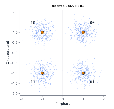
QPSK (quadrature phase-shift keying) sends two bits per symbol, one on I and one on Q. The four points sit at 45°, 135°, 225° and 315°. In this lesson the first (most significant) bit sets the sign of I and the second sets the sign of Q, with 0 as + and 1 as -:
| Bits | I | Q | Angle |
|---|---|---|---|
| 00 | +1 | +1 | 45° |
| 10 | -1 | +1 | 135° |
| 11 | -1 | -1 | 225° |
| 01 | +1 | -1 | 315° |
This is the mapping in figure 9 of the DVB-S2 standard (ETSI EN 302 307-1), which requires Gray-coded QPSK and labels the most significant bit I and the least significant bit Q.
Gray coding
Walk around the circle: 00, 10, 11, 01, back to 00. Each step changes exactly one bit. That is a Gray code. Noise moves a received point a small random distance, so the most likely wrong decision is a neighbouring point. With Gray coding that error costs one bit. With a natural binary order (00, 01, 10, 11 around the circle), two of the four neighbour pairs differ in both bits.
The receiver decides with two sign tests: I below zero gives a first bit of 1, Q below zero a second bit of 1. The mapper is two multiplexers:
assign i_sym = bits[1] ? -2'sd1 : 2'sd1;
assign q_sym = bits[0] ? -2'sd1 : 2'sd1;qpsk_mapper.sv
Pulse shaping
If you hold each symbol constant for its whole period, the I and Q waveforms are rectangular pulses. A rectangular pulse has a sinc-shaped spectrum with side lobes that fall off slowly, so the signal spills into neighbouring channels. Practical systems filter the symbols to confine the spectrum.
The filter must not smear one symbol into the next at the sampling instants. A pulse that is zero at the sampling instants of all other symbols causes no intersymbol interference (ISI). The raised-cosine family has that property. Its parameter, the roll-off factor α between 0 and 1, sets how much bandwidth the pulse uses beyond the minimum.
Root-raised cosine
The raised-cosine response is usually split in two equal halves: a root-raised-cosine (RRC) filter in the transmitter and another in the receiver. Together they form a raised cosine, so the ISI is zero after the receive filter. The receive half is also the matched filter, discussed at the end of the lesson.
DVB-S2 defines its RRC filter in the frequency domain (clause 5.6), with the Nyquist frequency fN = Rs/2:
- H(f) = 1 for |f| below fN(1 - α).
- H(f) = sqrt(1/2 + 1/2 sin(π (fN - |f|) / (2 fN α))) in the transition band.
- H(f) = 0 above fN(1 + α).
The standard allows α = 0.35, 0.25 or 0.20. This lesson uses 0.35. Because H(f) is zero above fN(1 + α), the baseband signal is (1 + α) Rs / 2 wide, and the passband signal occupies (1 + α) Rs around the carrier. At 12.5 MBd and α = 0.35 that is 16.875 MHz.
Taps for the FIR
qpsk_model.py computes the impulse response by numerically integrating the inverse Fourier transform of H(f). It samples the response at 8 samples per symbol over 6 symbols, which gives 6 × 8 + 1 = 49 taps. Two checks run in test_qpsk_model.py: the centre value matches the closed-form RRC peak 1 - α + 4α/π to within 1e-4, and a transmit and receive RRC pair leaves less than 0.2 % residual ISI. The residue comes from cutting the response off at 6 symbols.
The model then scales the taps to 16-bit integers and writes rrc_taps.hex, which the RTL loads with $readmemh (see memory and DSP for ROM files).
Upsampling and a filter without multipliers
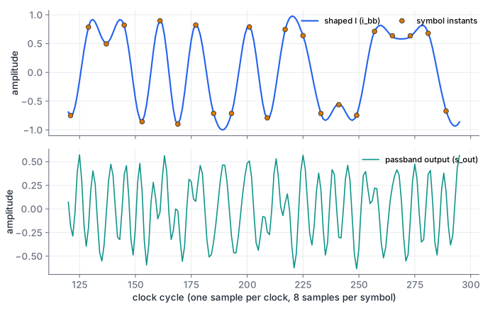
The FIR runs at the sample rate, 8 samples per symbol. The upsampler inserts the symbol value in one sample and seven zeros after it. The filter input is therefore always +1, -1 or 0, and each “product” is +tap, -tap or nothing:
always_comb begin
    acc = '0;
    for (int k = 0; k < NTAPS; k++) begin
        if (xs[k] == 2'sd1)       acc = acc + taps[k];
        else if (xs[k] == -2'sd1) acc = acc - taps[k];
    end
end
xs is a 49-stage delay line of 2-bit values. At any time at most 7 of its entries are non-zero, one per symbol in the 6-symbol window plus one at the edge. A polyphase filter would exploit that and add only those 7 taps; the direct form here is easier to read and still needs no multipliers.
The taps are scaled so that the worst-case sum, all non-zero inputs lined up with the taps of the same sign, is 32766. The output then always fits in 16 bits. Two’s complement wrap-around inside the accumulator cancels out when the final sum is in range, so a 16-bit accumulator is enough. test_qpsk_model.py checks the bound.
pulse_shaper.sv
Download rrc_taps.hex
I/Q modulation with an NCO
The mixer needs a cosine and a sine at the carrier frequency, sampled at the clock rate. That is a numerically controlled oscillator (NCO) built like the one in lesson 16: a 32-bit phase accumulator that adds a tuning word every clock. Here its top 8 bits address a full-cycle 256-entry Q1.15 sine table, not the quarter-wave table of lesson 16. The cosine is the same table read a quarter cycle (64 entries) ahead, so one ROM serves both.
The tuning word for a carrier fc at clock fclk is
For fc = 25 MHz and fclk = 100 MHz, TW = 2^30 = 0x4000_0000. At 12.5 MBd the passband reaches from 25 - 8.44 = 16.56 MHz to 33.44 MHz, well below the 50 MHz Nyquist limit of a 100 MS/s DAC.
The mixer is a three-stage pipeline:
phase <= phase + tuning_word;
cos_r <= sine[addr + 8'd64];          // stage 1: table look-up
sin_r <= sine[addr];
i_r   <= i_in;
q_r   <= q_in;
p_i   <= i_r * cos_r;                 // stage 2: products (DSP blocks)
p_q   <= q_r * sin_r;
s_out <= 16'(diff >>> 16);            // stage 3: difference, round, scale
diff is p_i - p_q + 32768. The two products are Q2.30 values of at most 32767² each, so their difference is below 2 × 32767², which is less than 2^31, and fits in 32 bits. Adding 2^15 before the 16-bit arithmetic shift rounds to nearest. The shift by 16 rather than 15 halves the amplitude, because |I cos - Q sin| can reach √2 times full scale.
The 8-bit table address drops the lower 24 phase bits. Lesson 16 shows how this phase truncation creates spurs, about 6 dB lower for each extra address bit.
Downloadnco_mixer.sv
The complete transmitter
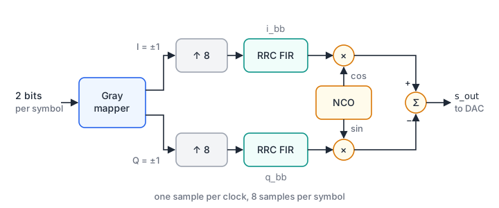
qpsk_tx.sv connects the blocks. A counter divides the clock by SPS = 8. The transmitter raises sym_ready in one clock of every eight and takes a symbol when sym_valid is also high. If no symbol is waiting, the filters receive zeros, so a gap in the data produces silence.
| File | Contents |
|---|---|
qpsk_mapper.sv | Gray mapping of 2 bits to I and Q of ±1 |
pulse_shaper.sv | 49-tap RRC FIR for one channel, add/subtract only |
nco_mixer.sv | Phase accumulator, sine table, I/Q mixer |
qpsk_tx.sv | Top level: symbol counter, upsampler, two filters, mixer |
qpsk_model.py | Bit-exact Python model; writes rrc_taps.hex and sine256.hex |
qpsk_tx.sv
Download sine256.hex
Download qpsk_model.py
Bit-exact verification with cocotb
A bit-exact model reproduces every output value of the hardware, including rounding, and here also the latency of each register. Counting clock edges after reset as e = 0, 1, 2 and so on, tx_reference() in qpsk_model.py computes:
i_bb[e]= the convolution of the filter input with the taps, at index e - 1 (one register after the delay line).s_out[e]= round((i_bb[e-3] C(e-2) - q_bb[e-3] S(e-2)) / 2^16), where C(m) and S(m) are the table entries addressed by the phase m × TW.
The model filters with NumPy’s convolve, not a delay line, so it is an independent implementation.
cocotb_qpsk_tx.py holds two tests. Each drives 4000 clock edges and compares i_bb, q_bb and s_out after every edge. The first offers a symbol in every slot with the carrier at 25 MHz. The second leaves 30 % of the slots empty and uses an arbitrary tuning word, 0x1234_5679. The test also checks that sym_ready is high in exactly one cycle of eight.
cd public/code/fpga-design/digital-modulation
python -m pytest -q
# 17 passed
The pytest wrapper test_cocotb_qpsk_tx.py builds the RTL with Icarus Verilog in a temporary directory, copies the hex files there for $readmemh, runs the cocotb module and fails if any cocotb test failed. The suite needs cocotb, NumPy and SciPy and runs in about 2 s.
The test catches real bugs. Removing the rounding constant in the mixer fails at the sixth edge (got 259, expected 260), and swapping the I and Q bits in the mapper fails at the second edge.
test_qpsk_model.py adds an end-to-end check. It demodulates the model’s s_out with an ideal receiver (same carrier phase, RRC matched filter, sampling at the known symbol instants) and recovers all 994 symbols of the test sequence.
cocotb_qpsk_tx.py
Download test_cocotb_qpsk_tx.py
Download test_qpsk_model.py
Bit errors in white noise
The usual first model of a channel adds white Gaussian noise (AWGN) with one-sided power spectral density N0. Performance is quoted against Eb/N0, the energy per bit divided by N0, usually in dB. Using Eb rather than the energy per symbol makes schemes with different bits per symbol comparable.
For BPSK, the receiver sees +√Eb or -√Eb plus Gaussian noise with variance N0/2. It decides on the sign. An error happens when the noise pushes the sample across zero, that is when the noise exceeds √Eb in the wrong direction:
Q(x) is the probability that a standard Gaussian variable exceeds x. Gray-coded QPSK is two independent BPSK signals, one on I and one on Q, each carrying one bit with energy Eb. Its bit error rate is the same function of Eb/N0, at twice the bits per symbol.
| Eb/N0 | 0 dB | 4 dB | 6.8 dB | 8 dB | 9.6 dB |
|---|---|---|---|---|---|
| Pb | 0.0786 | 0.0125 | 9.9e-4 | 1.9e-4 | 9.7e-6 |
ber.py checks the formula by Monte Carlo simulation. It draws random bits, maps them, adds seeded Gaussian noise with σ = √(N0/2), decides by the sign and counts errors. test_ber.py runs 2 million bits at 0, 2, 4, 6 and 8 dB for BPSK and at 0, 4 and 8 dB for QPSK. Each result must lie within five standard deviations of the binomial error count around the theory; at 8 dB that is about 380 expected errors.
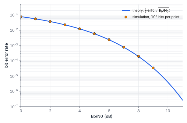
The steep slope is the practical lesson. From 1e-3 to 1e-5 costs only 2.8 dB. A small implementation loss, such as a filter with too few taps or a slightly wrong sample instant, therefore shows up as a large change in error rate. Forward error correction moves the curve further left; DVB-S2 combines LDPC and BCH codes for that.
Downloadber.py
Download test_ber.py
How a receiver recovers the symbols
The formula assumes a receiver that knows the carrier phase and the symbol timing exactly. A real receiver estimates both. Its main blocks are:
- Downconversion. Multiply the input by a local cosine and minus sine, as
coherent_receiver()inqpsk_model.pydoes. This produces I and Q plus components at twice the carrier, which the next filter removes. - Matched filter. Filter I and Q with the transmit pulse shape, here the same RRC. The matched filter maximises the signal-to-noise ratio at the sampling instant for white noise, and the RRC pair gives zero ISI.
- Symbol timing recovery. Find the instant within each symbol where the eye is most open, and track drift between the two clocks. A timing error detector estimates whether the current instant is early or late, and a loop steers an interpolator or the sample clock.
- Carrier recovery. The local oscillator is never exactly at the transmitter’s frequency or phase. A phase error rotates the constellation and pushes points toward the decision boundaries. A loop compares the received points with the nearest constellation points and corrects the NCO’s phase and frequency.
- Decision. Take the signs of I and Q.
The QPSK constellation looks the same after a 90° rotation, so a carrier loop can lock at any of four phases. Systems resolve this with known symbols (each DVB-S2 physical-layer frame starts with a 26-symbol start-of-frame field) or with differential coding.
Plan a transmitter configuration
Your board has a 100 MHz clock and a DAC that takes one sample per clock. You keep 8 samples per symbol but change the roll-off to α = 0.25 and the carrier to 20 MHz.
- What are the symbol rate, bit rate and occupied bandwidth?
- What tuning word do you need, and between which frequencies does the signal lie?
- Which parts of the design change?
Show solution
- Rs = 100 MHz / 8 = 12.5 MBd, so 25 Mbit/s with QPSK. The occupied bandwidth is (1 + 0.25) × 12.5 = 15.625 MHz.
- TW = round(20 / 100 × 2^32) = round(858 993 459.2) = 858 993 459 = 0x3333_3333. The actual carrier is 858 993 459 / 2^32 × 100 MHz = 19.999 999 995 MHz. The signal lies between 20 - 7.8125 = 12.19 MHz and 27.81 MHz.
- The tuning word is an input, so only the taps change. Set
ALPHA = 0.25inqpsk_model.pyand run it to rewriterrc_taps.hex. Thentest_qpsk_model.pyfails its ISI check: the impulse response decays more slowly, and with a 6-symbol span the residual ISI rises from 0.10 % to 3.1 %. WithSPAN = 16(129 taps) it falls to 0.05 %; setNTAPS = 129onqpsk_txto match.
Gray coding versus natural order
Suppose the mapper instead placed 00, 01, 10 and 11 at 45°, 135°, 225° and 315°.
- Which neighbouring pairs now differ in two bits?
- At high Eb/N0 nearly all symbol errors go to a neighbour, equally often in either direction. Roughly how does the bit error rate compare with the Gray mapping?
Show solution
- Going round the circle: 00 to 01 (one bit), 01 to 10 (two bits), 10 to 11 (one bit), 11 to 00 (two bits). Two of the four neighbour pairs differ in both bits.
- With Gray coding every neighbour error costs one bit. With the natural order, half of the neighbour errors cost two bits, so each symbol error costs 1.5 bits on average instead of 1. The bit error rate is about 1.5 times higher, which near 1e-5 costs about 0.2 dB of Eb/N0. The decision logic also gets harder: the bits are no longer the signs of I and Q.
Summary
- A modulator maps groups of bits to constellation points in the I/Q plane. BPSK carries 1 bit per symbol, QPSK 2. Gray coding makes neighbouring points differ in one bit.
- Root-raised-cosine filters in the transmitter and receiver together give zero intersymbol interference. With roll-off α, the passband signal occupies (1 + α) Rs.
- After zero-stuffing, the pulse-shaping FIR sees only +1, -1 or 0, so it adds and subtracts taps without multipliers. Scaling the taps for the worst case keeps the output inside 16 bits.
- An NCO with a tuning word TW = fc / fclk × 2^32 supplies cosine and sine; the mixer computes I cos - Q sin in three pipeline stages.
- A cocotb test compares every output sample with a bit-exact Python model, and a seeded simulation matches the BPSK error rate 0.5 erfc(√(Eb/N0)).
Check your understanding
Pick an answer for each question, then check. Answers stay hidden until you submit.
Further reading
- Standard
- Tool
Found a mistake or something unclear?Report a correction.
Follow this course
Get an email when new lessons and projects are added to this course.