Week 7 · Arithmetic and DSP · Lesson 15 of 24
FIR filters and CORDIC on FPGAs
Design FIR coefficients in Python, quantise them, build a transposed-form FIR in SystemVerilog, and compute sine, cosine and atan2 with a pipelined CORDIC.
What you will learn
- Design low-pass FIR coefficients with scipy.signal.firwin and quantise them to Q1.15
- Compare direct, transposed and systolic FIR structures and map them onto DSP slices
- Size the accumulator for bit growth and round and saturate the output once
- Explain CORDIC rotation and vectoring modes, the gain K and the iteration count
- Verify a filter and a pipelined CORDIC bit-exactly against a Python fixed-point model
Before you start
- FPGA memory and DSP (lesson 14)
- Python testbenches with cocotb (lesson 10)
- Static timing analysis and timing closure (lesson 11)
After this lesson you can take a filter specification, design the coefficients in Python, turn them into fixed-point integers, and build a pipelined FIR filter that maps onto DSP slices. You will also build a CORDIC, the shift-and-add algorithm that computes sine, cosine, arctangent and vector magnitude without a multiplier. Both designs are checked bit for bit against a Python model.
The building blocks come from FPGA memory and DSP: Q1.15 arithmetic, rounding, saturation and the multiply-accumulate. In the semester project, this filter cleans up samples that arrive over the UART, and the CORDIC returns in the DDS lesson.
FIR filter basics
A finite impulse response (FIR) filter computes each output sample as a weighted sum of the current and previous input samples:
The weights are the coefficients, also called taps. N is the number of taps. One output costs N multiplications and N - 1 additions.
Feed the filter an impulse (a single 1 followed by zeros) and the output is the coefficient sequence. This impulse response is finite: after N samples it is zero again. The output for any input is the convolution of the input with the impulse response, so the coefficients set which frequencies pass.
FIR filters have no feedback, so they are always stable and pipeline easily. With symmetric coefficients, , they have linear phase: every frequency is delayed by the same samples, so the shape of a pulse is preserved.
Designing coefficients in Python
Coefficient design is a software job. scipy.signal.firwin designs a windowed-sinc filter from a tap count and a cutoff frequency. The example is a 31-tap low-pass for audio sampled at 48 kHz, with the cutoff at 6 kHz:
from scipy import signal
import numpy as np

h = signal.firwin(31, 6000.0, fs=48000.0)          # Hamming window by default
h_q = np.clip(np.round(h * 2**15), -32768, 32767)   # quantise to Q1.15
Three details from the SciPy documentation matter here. The default window is Hamming. The cutoff is the half-amplitude (-6 dB) point, not a -3 dB point. With the default scale=True, the gain at DC is exactly 1, so the coefficients sum to 1.
Quantising to fixed point
The hardware needs integers. Multiply each coefficient by and round to get Q1.15. The largest coefficient here is 0.2507, which becomes 8216. Six of the 31 quantised coefficients are exactly zero. The cutoff is one eighth of the sample rate, so the ideal impulse response at offset m from the centre tap is . It is zero for m = ±4, ±8 and ±12.
Quantisation changes the frequency response. The figure compares the floating-point design with 16-bit and 8-bit coefficients.
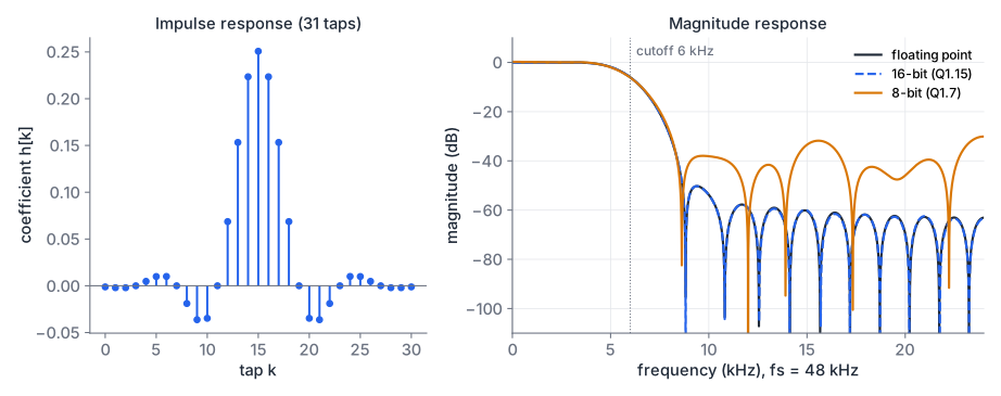
With Q1.15 coefficients the response is indistinguishable from the floating-point design. The worst stop-band level above 9 kHz is -50.3 dB in both cases. With 8-bit Q1.7 coefficients it is -30.1 dB, because the small outer coefficients round to 0 or 1. Always check the quantised response before you choose a coefficient width.
fir_model.py contains this design, the quantisation and a bit-exact model of the hardware. Run standalone, it prints the packed coefficient literal used as the RTL default.
Bit growth and output scaling
Each product of a Q1.15 sample and a Q1.15 coefficient is a 32-bit Q2.30 number. Adding N of them can grow the result by up to bits. For 31 taps that is 5 bits, so a 37-bit accumulator can hold any possible sum without overflow. The RTL computes this width from the parameters:
localparam int PW = DW + CW;              // product width: 32
localparam int AW = PW + $clog2(NTAPS);   // accumulator width: 37
A tighter bound uses the actual coefficients. The worst-case output is the full-scale input times . For this filter . A DC input comes out at a gain of about 1 (32770/32768 after quantisation), but an input whose signs follow the signs of the coefficients comes out 1.38 times larger than full scale (+2.8 dB). The output therefore needs saturation.
Keep the full precision through the whole sum and round once at the end. Lesson 14 showed the Q1.15 rounding: add (half an output LSB), shift right arithmetically by 15, then saturate to the 16-bit range. Rounding after every product would add N rounding errors instead of one.
FIR structures and DSP slices
The same equation can be built in several ways, with different timing, latency and fit to the DSP slices.
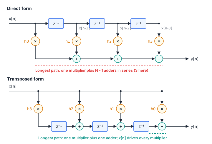
Direct form. A shift register holds the last N samples, each tap multiplies one of them, and an adder chain or tree sums the products. Without extra pipelining, the longest path contains a multiplier and every adder. An adder tree shortens it to adder levels. UG479 notes that in this structure the fabric adders are usually the performance bottleneck.
Transposed form. Reverse the direction of the signal flow and swap the input and output, and the delays move into the adder chain. Every multiplier now sees the same current sample. Each partial sum is registered before the next tap adds its product, so a register-to-register path holds one multiplier and one adder regardless of N. The cost is fanout: the input register drives all N multipliers, and for long filters that wide net can become the critical path instead.
Systolic form. The DSP48E1 slice in AMD 7-series devices can pass its 48-bit result to the next slice in the column over a dedicated cascade (PCOUT to PCIN), without leaving the slice. UG479 recommends building pipelined filters on these adder cascades rather than on fabric adder trees. In the systolic FIR of UG479 Figure 3-6, the input moves through two registers per tap while the partial sum moves through one, so the sample and the sum stay aligned. Every path is local. Latency grows with the number of taps.
Using symmetry: the pre-adder
A linear-phase filter has . In the direct and systolic forms, the two samples that share a coefficient can be added first and multiplied once:
That halves the multipliers: a 31-tap filter needs 16 (15 pairs plus the centre tap). The DSP48E1 has a 25-bit pre-adder in front of its 25 x 18 multiplier for this purpose, and UG479 shows it in an 8-tap even-symmetric systolic FIR. Other DSP block families have their own pre-adder options, so check the DSP user guide for your device. The pre-adder output is one bit wider than the samples, so 16-bit samples become 17 bits before the multiplier.
In the transposed form, the two taps that share a coefficient see the same sample, so and are the same product. One multiplier can feed both adders, and no pre-adder is needed.
The transposed FIR in SystemVerilog
fir_transposed.sv is parameterised by the tap count, the widths and a packed coefficient vector. It has four register stages, each matching a register inside a DSP slice: the input, the products, the partial sums, and the rounded output. The heart of it is the adder chain:
// Stage 3: transposed adder chain. It holds the filter state, so it is
// reset and only advances when a valid product arrives.
always_ff @(posedge clk) begin
    if (rst) begin
        for (int k = 0; k < NTAPS; k++) s[k] <= '0;
    end else if (v2) begin
        for (int k = 0; k < NTAPS - 1; k++) begin
            s[k] <= AW'(m[k]) + s[k+1];
        end
        s[NTAPS-1] <= AW'(m[NTAPS-1]);
    end
end
After the update, s[0] holds for the newest sample. The chain only moves when a valid product arrives, so idle cycles between samples do not shift the filter state. The latency from in_valid to out_valid is 4 clock cycles, and the filter accepts a new sample every cycle. Because the coefficients are parameters, each multiplier has a constant operand. Synthesis removes the multipliers of the zero taps (their delay registers stay), and it may implement some constant multiplications with shifts and adds in LUTs instead of DSP slices. Read the utilisation report to see what it chose.
fir_transposed.sv
Download fir_model.py
Bit-exact verification
The model uses exact integer convolution and the same round-and-saturate step as the RTL, so the outputs must match exactly. Any difference is a bug.
cocotb_fir.py runs four tests, using the method from the cocotb lesson: an impulse that must return the quantised coefficients, 600 random full-range samples with random gaps in in_valid, a worst-case pattern that drives the output into saturation in both directions, and a two-tone signal. The pytest wrapper builds the design twice, once with the 31-tap default and once with a 7-tap filter passed in through the parameters.
cocotb_fir.py
Download test_cocotb_fir.py
Download test_fir_model.py
# needs Python with cocotb, NumPy, SciPy and pytest, plus Icarus Verilog
cd fir-filters-and-cordic
python -m pytest -q
# 18 passed  (model tests plus the cocotb runs of both designs)
CORDIC
CORDIC (COordinate Rotation DIgital Computer) rotates a vector through a sequence of fixed angles using only additions, subtractions and shifts. Jack Volder developed it in the 1950s for aircraft navigation. It suits FPGAs because a shift by a constant amount is just wiring.
The idea
Rotating a vector by an angle needs four multiplications:
Factor out and the rest depends only on . CORDIC restricts the rotation angles to , so multiplying by becomes a right shift by i bits. Iteration i rotates by :
Here is the direction, and z tracks the angle. The angles are 45°, 26.565°, 14.036°, 7.125° and so on, roughly halving each time, so each iteration adds about one bit of precision.
The gain K
Dropping the factor means each iteration lengthens the vector by . After n iterations the length has grown by , where
K converges quickly. The model computes , and , so the gain is . The scale does not depend on the directions , so it is a constant for a fixed iteration count. You correct it once, either by starting with a vector of length K or by scaling the result.
Rotation mode: sine and cosine
In rotation mode, z starts at the target angle and each iteration chooses to drive z towards zero: if , else . Start with and the final vector is .
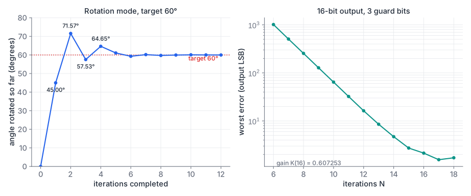
Worked example, , starting from without the K correction:
| i | Angle rotated so far | Residual z | x | y | ||
|---|---|---|---|---|---|---|
| 0 | 45.000° | +1 | 45.000° | 15.000° | 1.0000 | 1.0000 |
| 1 | 26.565° | +1 | 71.565° | -11.565° | 0.5000 | 1.5000 |
| 2 | 14.036° | -1 | 57.529° | 2.471° | 0.8750 | 1.3750 |
| 3 | 7.125° | +1 | 64.654° | -4.654° | 0.7031 | 1.4844 |
| 4 | 3.576° | -1 | 61.077° | -1.077° | 0.7959 | 1.4404 |
| 5 | 1.790° | -1 | 59.288° | 0.712° | 0.8409 | 1.4156 |
After eight iterations the vector is (0.8300, 1.4223). Multiplying by gives (0.5040, 0.8637), against the exact (0.5, 0.8660). Sixteen iterations bring the error down to the last bit of a 16-bit result.
Range
The angles add up to 99.88°, so the iterations can only reach targets within about ±99.9°. For a full circle, first rotate by ±90°, which costs nothing: is a swap and a negation. After that pre-rotation, the residual angle is always within ±90°.
Vectoring mode: atan2 and magnitude
In vectoring mode, the input is a vector and z starts at zero. Each iteration chooses to drive y towards zero: if , else . When y reaches zero, the vector lies on the x axis. Then z holds the angle the vector was rotated through, which is , and x holds the magnitude , scaled by . Inputs with get the same ±90° pre-rotation first.
Worked example, . After the first iteration (d = -1, rotate by -45°) the vector is (7.0, 1.0) and the accumulated angle is 45°. After the second it is (7.5, -2.5) at 71.57°, after the third (8.125, -0.625) at 57.53°. After 16 iterations, z = 53.129° (exact: 53.130°) and x = 8.2338. Multiplied by , the magnitude is 5.0000. cordic_vector() in the model prints the full trace.
A pipelined CORDIC in SystemVerilog
An iterative CORDIC reuses one shift-add stage N times, which needs variable shifters. Andraka’s survey notes that wide variable shifters map poorly onto FPGA logic. Unrolling the loop gives each stage a fixed shift, which is just wiring, and a fixed angle constant. Andraka also points out that most FPGA architectures already have a register in every logic cell, so the pipeline registers cost no extra logic. cordic.sv is that unrolled, pipelined design:
- Input: a 16-bit binary angle, . The angle wraps naturally at ±180°, and the quadrant is in the top two bits.
- Stage 0: the ±90° pre-rotation, starting from , which builds the gain correction into the start value.
- Stages 1 to N: one iteration each, N = 16 by default.
- Output stage: round away the 3 guard bits and saturate to 16 bits.
Internally x and y are 20 bits wide: 16 output bits, 3 guard bits that reduce the error from truncated shifts, and 1 bit of headroom. The angle path is 20 bits, so the arctangent table holds , rounded. One iteration:
for (genvar i = 0; i < N; i++) begin : g_stage
    always_ff @(posedge clk) begin
        if (!z[i][ZW-1]) begin                  // z >= 0: rotate counter-clockwise
            x[i+1] <= x[i] - (y[i] >>> i);
            y[i+1] <= y[i] + (x[i] >>> i);
            z[i+1] <= z[i] - atan_tab(i);
        end else begin                          // z < 0: rotate clockwise
            x[i+1] <= x[i] + (y[i] >>> i);
            y[i+1] <= y[i] - (x[i] >>> i);
            z[i+1] <= z[i] + atan_tab(i);
        end
    end
end
The latency is N + 2 = 18 clock cycles, and a new angle enters every cycle. Each stage holds three 20-bit adder-subtractors (x, y and angle) and no multiplier. Python’s >> on integers floors exactly like >>> on signed values, so the model matches the hardware bit for bit.
cordic.sv
Download cordic_model.py
Download cocotb_cordic.py
Download test_cocotb_cordic.py
Download test_cordic_model.py
Download tb_cordic.sv
The cocotb tests check the latency, the quadrant boundaries, every 16th angle around the circle and 1500 random angles with idle gaps, all bit-exact against cordic_model.py. The model tests confirm that the RTL constants match the model and that the error over all 65536 angles is at most 2.33 LSB. For readers without Python, tb_cordic.sv streams all 65536 angles and checks them against $cos and $sin with a 3 LSB limit:
iverilog -g2012 -o sim tb_cordic.sv cordic.sv && vvp sim
# 65536 angles checked, worst error 2.332954 LSB
# PASSSize a symmetric filter for a 12-bit ADC
A 63-tap linear-phase low-pass filter takes samples from a 12-bit ADC and uses 18-bit coefficients. It will be built in systolic form on DSP48E1 slices with the pre-adder.
- How many multipliers does it need?
- How wide is the pre-adder output, and does it fit the multiplier port it feeds?
- How wide must the accumulator be so that no sum can overflow?
Show solution
- 63 taps form 31 pairs plus the centre tap, so 32 multipliers (32 DSP slices).
- Adding two 12-bit signed samples needs 13 bits. That fits easily in the 25-bit pre-adder and the 25-bit multiplier input, and the 18-bit coefficient fits the 18-bit port.
- Each product is at most 13 + 18 = 31 bits. Thirty-two products add bits, so 36 bits are enough. That fits in the slice’s 48-bit accumulator and cascade.
Four CORDIC iterations by hand
Compute and with four rotation-mode iterations, starting from . Use the angles 45°, 26.565°, 14.036° and 7.125°. Correct the result with and compare it with the exact values.
Show solution
| i | Residual z after | x | y | |
|---|---|---|---|---|
| start | -40.000° | 1 | 0 | |
| 0 | -1 | 5.000° | 1 | -1 |
| 1 | +1 | -21.565° | 1.5 | -0.5 |
| 2 | -1 | -7.529° | 1.375 | -0.875 |
| 3 | -1 | -0.404° | 1.265625 | -1.046875 |
The vector now points at -39.596°. Scaled by 0.60883: and , against the exact 0.7660 and -0.6428. The 0.4° residual angle accounts for the error.
Summary
- An FIR filter is a convolution of the input with N coefficients. Design them in Python with
firwin, quantise to fixed point, and check the quantised frequency response: 16-bit coefficients matched the floating-point design here, 8-bit ones lost 20 dB of stop band. - Products of Q1.15 values are Q2.30. Summing N of them adds up to bits. Keep full precision, then round and saturate once at the output.
- The direct form sums the products in a long adder chain or tree. The transposed form has one multiplier and one adder per path but a high-fanout input. The systolic form uses the DSP cascade and keeps every path local, at the cost of latency.
- Symmetric coefficients halve the multipliers, through a pre-adder in direct and systolic forms or a shared product in the transposed form.
- CORDIC rotates by using shifts and adds. Rotation mode gives sine and cosine, vectoring mode gives atan2 and magnitude, the gain is a constant, and each iteration adds about one bit.
- Fixed-point designs can be verified bit-exactly against an integer Python model. Any mismatch is a bug, not a tolerance question.
Check your understanding
Pick an answer for each question, then check. Answers stay hidden until you submit.
Further reading
- Book
- Paper
- Paper
- Documentation
- Tool
Found a mistake or something unclear?Report a correction.
Follow this course
Get an email when new lessons and projects are added to this course.