Week 11 · AI on FPGAs · Lesson 23 of 24
AI inference on FPGAs: INT8 quantisation and systolic arrays
Run a quantised network layer in FPGA fabric: INT8 scales and zero points, requantisation with a multiplier and shift, systolic MAC arrays, hls4ml and FINN.
What you will learn
- Explain when an FPGA is a good inference target in terms of latency, determinism and custom precision
- Quantise a fully connected layer to INT8 with per-channel weight scales and an INT32 bias
- Implement requantisation with a fixed-point multiplier and a rounding shift, bit-exact with a Python model
- Describe weight-stationary and output-stationary dataflows and map a layer onto an N x N systolic array
- Estimate cycles and on-chip memory bandwidth for a layer and choose between hand-written RTL, hls4ml, FINN and vendor AI tools
Before you start
- FPGA memory and DSP: block RAM, FIFOs and MACs (lesson 14)
- Verification with cocotb (lesson 10)
- INT8 quantisation basics, covered in the Robotics and AI course lesson on deployment
After this lesson you can take a small trained network layer, quantise it to 8-bit integers, and run it in FPGA fabric with results that match a Python model bit for bit. You will build the two blocks every INT8 accelerator needs: a systolic array of multiply-accumulate (MAC) units and a requantisation stage that turns 32-bit sums back into 8-bit activations.
The arithmetic builds on the MAC and fixed-point material in memory and DSP. The quantisation formulas themselves are introduced in the Robotics and AI lesson on deployment and safety. Read its INT8 section first if scale and zero point are new to you. This lesson starts where that one stops: what the integer arithmetic looks like in hardware.
Why run inference on an FPGA
A CPU or GPU runs a network as a sequence of instructions over memory. An FPGA can instead lay the network out as a pipeline of dedicated multipliers, adders and RAMs. Three properties follow.
- Latency. With every layer in fabric and the weights in on-chip memory, there is no instruction fetch, no operating system and no off-chip memory round trip. The hls4ml case study by Duarte et al. fitted a jet-classification network for a particle-physics trigger on an FPGA with a latency of about 100 ns.
- Determinism. A pipeline built from registers has a fixed latency in clock cycles. The systolic array in this lesson always produces a tile 2N - 1 cycles after its last input beat. A control loop or a trigger system can budget for that number exactly.
- Custom precision. Fabric multipliers can be any width. hls4ml lets you choose the fixed-point width. FINN goes to the extreme: Umuroglu et al. map binarised networks, with 1-bit weights and activations, onto XNOR and popcount logic.
The costs are longer design time and a less flexible deployment: a model that changes every week is easier to run on a processor. FPGAs pay off when latency, power or determinism matter most, or when the inference sits next to other FPGA logic such as a camera pipeline.
INT8 arithmetic for hardware
The affine mapping
Jacob et al. define the quantisation scheme adopted in TensorFlow Lite. A real value is represented by an integer with a scale and a zero point :
The current LiteRT (TensorFlow Lite) 8-bit specification fixes the details that matter for hardware:
- Activations: INT8 in , asymmetric, so the zero point can be anywhere in that range.
- Weights: INT8 in , symmetric with , and one scale per output channel (“per-axis”) for convolutions.
- Bias: INT32 with scale and zero point 0, so it adds straight into the accumulator.
Per-channel weight scales cost almost nothing in hardware. The scale only appears at requantisation, once per output, and the requantisation unit takes its multiplier as an input.
The integer layer
A fully connected layer computes . Substituting the quantised forms (with ):
Expand the bracket. The term depends only on the weights, so it is a constant per output channel. Jacob et al. use the same expansion to keep zero points out of the inner loop. Fold it into the bias offline:
The array now multiplies plain INT8 numbers. Each product fits in 16 bits: the largest magnitude is . An INT32 accumulator therefore holds worst-case products without overflow, far more than the 64 inputs of the example.
Requantisation: multiplier and shift
The output is INT8 again, with its own scale and zero point :
is a real number. Jacob et al. report that it is always in in practice and write it as with . Stored as a 32-bit integer, is at least , so it keeps at least 30 bits of relative precision. The multiplication by becomes a shift that must round to nearest.
In this lesson m0 is the integer and shift is . The whole requantisation is:
with , or to apply a ReLU (real value 0 maps to ). The rounding here is round half up. Frameworks differ in how they break exact ties. If you need bit-exact agreement with a specific framework, copy its rounding function, and test it the way the cocotb tests below do.
def quantize_multiplier(m: float) -> tuple[int, int]:
    frac, exp = math.frexp(m)          # m = frac * 2^exp, 0.5 <= frac < 1
    m0 = round(frac * (1 << 31))
    if m0 == 1 << 31:                  # rounding reached 1.0: renormalise
        m0 //= 2
        exp += 1
    return m0, -exp                    # shift = -exp

def requantize(acc, bias, m0, shift, zp, relu=False) -> int:
    p = (acc + bias) * m0
    r = (p + (1 << (30 + shift))) >> (31 + shift)   # round half up
    return max(zp if relu else -128, min(127, r + zp))
requant.sv
The RTL has three pipeline stages. Stage 1 adds the bias in 33 bits, so acc + bias cannot overflow. Stage 2 forms the full 65-bit product. Stage 3 adds the rounding constant, shifts, adds the zero point and saturates:
always_comb begin
    half    = 65'sd1 <<< (30 + int'(sh2));
    shifted = (prod2 + half) >>> (31 + int'(sh2));
    y       = shifted + 65'(zp2);
    lo      = relu2 ? 65'(zp2) : -65'sd128;
end

always_ff @(posedge clk) begin
    if (y > 65'sd127)  q <= 8'sd127;
    else if (y < lo)   q <= lo[7:0];
    else               q <= y[7:0];
end
Because m0, shift and zp are inputs, one instance serves all output channels: feed each accumulator together with its channel’s parameters. The 33 x 32-bit multiply is larger than one DSP slice (25 x 18 bits in AMD 7-series devices, up to 27 x 27 in Intel variable-precision blocks). Synthesis splits it across several slices, and you may want an extra pipeline register for timing at high clock rates.
requant.sv
Systolic arrays
H. T. Kung’s 1982 paper explains systolic architectures, a concept first proposed for VLSI implementation of matrix operations, around one observation: if a data item is fetched from memory once and then used by many processing elements as it is pumped from cell to cell, throughput can rise without more memory bandwidth. His Figure 1 makes the point with numbers: a memory with a 100 ns cycle feeding one processing element limits it to 5 million operations per second; the same memory feeding a chain of six cells allows 30 million.
Dataflows
Matrix multiplication is the natural fit. Each output needs a row of A and a column of B, and every A value is used by every column. The question is what stays still in each processing element (PE). Sze et al. name the common choices:
- Weight stationary: each weight is loaded into a PE once and stays there. Inputs stream through, and partial sums move from PE to PE. This minimises the energy spent reading weights. Kung’s design B1 (“broadcast inputs, move results, weights stay”) is an early example.
- Output stationary: each PE keeps the partial sum of one output. Inputs and weights stream past. This minimises the energy of reading and writing partial sums. Kung’s design B2 (“broadcast inputs, move weights, results stay”) is of this kind.
The reason the choice matters is energy and bandwidth. In the memory hierarchy figure of Sze et al., a DRAM access is shown at about 200 times the energy of a register-file access next to the arithmetic unit. Every byte that stays in a PE register is a byte not fetched from further away.
The array in this lesson
systolic_array.sv is an output-stationary N x N array. It computes one N x N tile of , with INT8 operands and INT32 accumulators.
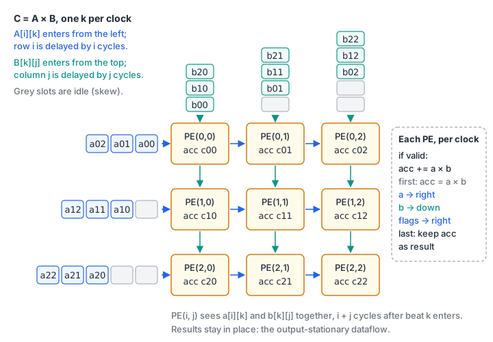
Each clock, column of A enters on the left and row of B on the top. Row is delayed by cycles and column by cycles. A value then needs more cycles to reach column , and a B value more cycles to reach row , so both reach PE exactly cycles after they entered. Flags for valid, first and last travel with the A values. The core of each PE:
assign prod = a_h[i][j] * b_v[i][j];                         // 16-bit signed
assign sum  = (f_h[i][j][1] ? 32'sd0 : acc) + 32'(prod);   // first beat restarts

always_ff @(posedge clk) begin
    if (f_h[i][j][0]) begin                 // valid
        acc <= sum;
        if (f_h[i][j][2]) res[i][j] <= sum; // last: keep the result
    end
end
The data registers have no reset, as in the MAC of lesson 14; only the flag pipeline is reset. PE finishes last, cycles after the last beat, and its done flag drives out_valid. The interface rule follows: a new tile’s last beat must come at least cycles after the previous one, or PE overwrites its result before out_valid. For tiles can run back to back with no idle cycles.
systolic_array.sv
Bandwidth
Per cycle the array reads INT8 operands and performs MACs. Each operand is used times. For that is 32 bytes per cycle for 256 MACs. Those bytes come from block RAM, so the design question becomes how many block RAM ports you need and how wide they are. Kung’s point applies directly: a larger array needs more compute but its memory traffic grows only with .
The other memory question is capacity. A fully parallel design such as the hls4ml case study keeps every weight on chip, in the programmable logic. If the weights do not fit, they stream from external memory, and the external bandwidth sets the speed. Count the weight bytes before choosing an architecture.
Worked example: an INT8 digit classifier
int8_layer.py builds a small, reproducible problem. It draws ten 8 x 8 seven-segment style digit glyphs, then makes noisy copies with random one-pixel shifts, random stroke intensity and Gaussian noise (), all from a fixed seed. There are 1500 training images and 500 test images. No external dataset is downloaded.
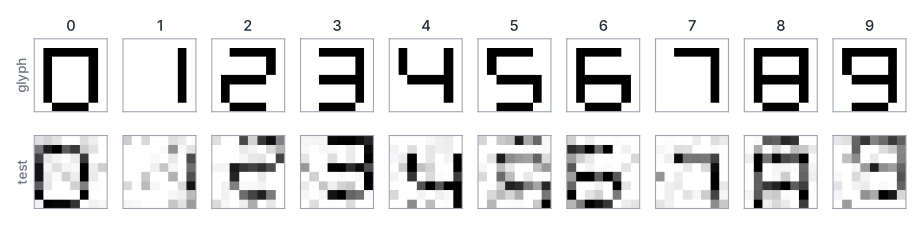
A linear classifier (64 inputs, 10 outputs) is trained in floating point with NumPy. The script then quantises it as described above:
- inputs: pixels in with and ,
- weights: per-channel symmetric INT8,
- bias: INT32 with the input zero point folded in,
- outputs: INT8 with a scale and zero point calibrated on the training logits.
$ python int8_layer.py
test samples: 500
float accuracy: 0.932   int8 accuracy: 0.928   same class: 0.996
input  scale 1/255, zero point -128
output scale 0.08733, zero point 8
weight scales: [0.02519 0.01719 0.02143 0.01809 0.02133 0.02594 0.02525 0.01962 0.01412
 0.01767]
channel 0: M = 1.131267e-03 -> m0 = 1243841297, shift = 9
largest |accumulator| = 241526
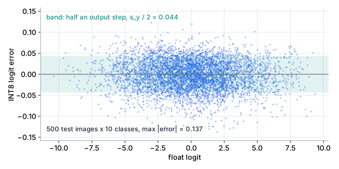
The INT8 layer picks the same class as the float layer for 99.6 % of the test images. Accuracy drops by 0.4 percentage points. The largest accumulator, 241526, uses 19 bits of the 32 available.
Mapping the layer onto the array
The layer is a matrix product: a batch of images (M x 64) times the transposed weights (64 x 10). On a 4 x 4 array, 8 images and 10 outputs (padded to 12 with zero weights) make 2 x 3 = 6 tiles. Each tile streams beats, so the 6 tiles take 384 cycles plus 7 cycles of latency, and the array does 16 MACs per cycle. The accumulators then go through requant.sv, one per cycle, with each channel’s bias, m0 and shift.
Verification
The cocotb tests compare the RTL with the Python model bit for bit.
cocotb_systolic.pysends 60 random tiles with from 1 to 40, about 30 % extreme values (, and others) and random idle cycles. It also tests tiles at the minimum spacing , the largest-magnitude cases, and the classifier layer itself, checking every accumulator againstint_matmul.cocotb_requant.pychecks 4360 values, including the INT32 limits foraccandbias, the extremem0andshiftvalues and both ReLU settings, againstrequantize. It then checks that the classifier accumulators of 40 images produce exactly the INT8 logits of the Python model.
cd public/code/fpga-design/ai-inference-on-fpgas
/Volumes/M2-Dev/conda/envs/toptech/bin/python -m pytest -q
# 11 passed
The pytest wrapper builds each module with Icarus Verilog in a temporary directory and fails if any cocotb test fails. Removing the rounding constant or the first restart from the RTL makes the suite fail.
int8_layer.py
Download test_int8_layer.py
Download cocotb_systolic.py
Download cocotb_requant.py
Download test_cocotb_ai.py
Tools that generate the hardware
Hand-written RTL gives full control and shows what the hardware does. For whole networks, generators save a lot of work.
- hls4ml translates trained models into high-level synthesis (HLS) code. Duarte et al. describe the flow for Keras and PyTorch models, fixed-point arithmetic with a configurable width, and a “reuse factor” : each multiplier is used times per layer, so is fully parallel and larger trades latency for fewer multipliers. The current documentation lists Keras, PyTorch and ONNX front ends (with quantised variants such as Brevitas and QONNX) and several back ends, including AMD Vivado/Vitis, Altera and Catapult.
- FINN, from AMD’s research labs, generates a dataflow architecture tailored to each quantised network. The original paper used a heterogeneous streaming architecture, with compute resources per layer sized to a throughput target and parameters kept on chip. On a ZC706 board it reported up to 12.3 million MNIST classifications per second at 0.31 µs latency for a binarised network.
- Vendor AI tools usually take a different route: a fixed, configurable neural-network processor plus a compiler, rather than a custom circuit per network. AMD describes Vitis AI as an inference development platform for its adaptive SoCs, with a compiler, a neural processing unit (NPU) IP, runtime software and the Quark quantiser; the current release lists general access support for the Versal AI Edge Series and its Gen 2. Microchip’s VectorBlox Accelerator SDK compiles quantised INT8 TFLite models for AI/ML inference on PolarFire FPGAs and PolarFire SoC FPGAs. Supported device lists change between releases, so check the vendor page.
Whichever tool you use, the checks in this lesson still apply: confirm the accumulator width, the rounding of the requantisation, and the accuracy of the quantised model on held-out data.
Requantise by hand
An output channel has and output zero point . Find m0 and shift. Then requantise an accumulator of 10000 with bias . Finally requantise an accumulator of (bias 0) without and with ReLU.
Show solution
math.frexp(0.0123) gives , so shift = 6 and m0 = round = 1690499128. Check: .
. The real product is , which rounds to 117. Adding gives . The integer path: ; adding and shifting right by 37 gives 117. requantize(10000, -500, 1690499128, 6, 8) returns 125.
For : , plus 8 is , which saturates to . With ReLU the lower clamp is , so , which dequantises to exactly 0.
Size an array for a larger layer
A layer has 784 inputs and 128 outputs. You process batches of 16 images on a 16 x 16 output-stationary array with the interface of systolic_array.sv. How many tiles are there, how many cycles does a batch take, and how many weight bytes must be on chip? Assume a 200 MHz clock and give the batch time.
Show solution
Tiles: , each with beats. Since , the tiles run back to back: cycles, plus 31 cycles until the last out_valid, so 6303 cycles. At the assumed 200 MHz that is about 31.5 µs per batch of 16 images.
Check with MAC counts: MACs, divided by 256 MACs per cycle, is 6272 cycles. The array is fully used while streaming.
Weights: bytes (about 98 KiB) of INT8, plus 128 INT32 biases and the per-channel m0 and shift. Compare this with the block RAM of your device. Each cycle reads 16 weight bytes and 16 input bytes, so the weight store must deliver 128 bits per cycle.
Summary
- FPGAs suit inference when latency, determinism, power or custom precision matter more than peak throughput.
- INT8 inference keeps INT8 x INT8 products in INT32 accumulators. Symmetric per-channel weights and an asymmetric input zero point folded into the INT32 bias keep the inner loop a plain integer MAC.
- Requantisation multiplies by as an integer
m0in Q0.31 and a rounding right shift, then adds the output zero point and saturates. - Systolic arrays reuse each fetched operand N times. Weight-stationary arrays keep weights in the PEs; output-stationary arrays, like the one here, keep partial sums.
- Verify against an integer Python model bit for bit, including extreme values, idle cycles and the tile spacing rule.
- hls4ml and FINN generate per-network hardware; vendor AI suites compile networks onto a configurable processor IP.
Check your understanding
Pick an answer for each question, then check. Answers stay hidden until you submit.
Further reading
- Paper
- Paper
- Paper
- Paper
- Paper
- Tool
- Documentation
Found a mistake or something unclear?Report a correction.
Follow this course
Get an email when new lessons and projects are added to this course.