Week 9 · Video and image processing · Lesson 20 of 24
Streaming image processing on an FPGA: Sobel edges
Process video one pixel per clock: grayscale in fixed point, line buffers in block RAM, a 3x3 window, Sobel edges, border handling, latency and a NumPy check.
What you will learn
- Explain when a streaming pipeline can replace a frame buffer, and what it costs in memory and latency
- Convert RGB to grayscale with integer BT.601 weights and bound the rounding error
- Build line buffers in block RAM and a 3x3 window generator for raster-order pixels
- Implement the Sobel operator with the |Gx| + |Gy| magnitude, a threshold and defined border behaviour
- Verify the pipeline bit-exactly against a NumPy reference with cocotb
Before you start
- Memory and DSP (lesson 14)
- Video timing and HDMI (lesson 19)
- Verification with cocotb (lesson 10)
In this lesson you build an edge detector that processes video as it arrives, one pixel per clock, with only two lines of memory. You will convert RGB to grayscale in fixed point, store lines in block RAM, assemble a 3×3 window, compute Sobel gradients, and check every output pixel against a NumPy reference.
The pixels arrive in the raster order of video timing and HDMI, and the line buffers use the block RAM templates from memory and DSP.
Streaming versus a frame buffer
There are two ways to organise an image pipeline.
A frame buffer design writes the whole frame to memory, then reads it back in any order. It can do anything, but the memory is large. A 640 × 480 RGB frame with 8 bits per colour is 640 × 480 × 24 = 7 372 800 bits. That is exactly 200 block RAMs of 36 Kb (36 864 bits) each, more than many small FPGAs have, so frame buffers usually live in external DRAM. That adds a memory controller, bandwidth limits and latency of at least a frame.
A streaming design processes pixels in the order they arrive and never stores the whole frame. It works for any operation whose output pixel depends only on input pixels close to it: point operations (colour conversion, thresholds, gamma) and small neighbourhoods (blur, sharpening, edge detection). A 3×3 neighbourhood needs the current line and the two before it, so it stores two lines: 2 × 640 × 8 = 10 240 bits for 8-bit gray, about a quarter of one 36 Kb block RAM.
Operations that need distant pixels do not fit this model. Rotating an image by 90° makes the first input column the first output line, so the full frame must be stored before the first output pixel. A histogram can be collected while streaming, but applying a correction based on it to the same frame needs that frame stored.
Streaming has a second benefit: latency. The edge detector in this lesson produces its result about one line after the input, 31.8 µs at 640 × 480 and 60 Hz.
Raster order and the stream interface
Pixels enter in raster order: left to right, then top to bottom. The pipeline uses a simple interface:
| Signal | Meaning |
|---|---|
in_valid | A pixel is present this clock |
in_sof | This pixel is (0, 0), the start of a frame |
r, g, b | 8-bit colour |
in_valid may have gaps, for example during video blanking (DE low) or when an upstream block stalls. The pipeline advances only on valid pixels. Every input pixel produces exactly one output pixel with out_valid, out_sof, an 8-bit magnitude mag and a 1-bit edge_out, six clocks later. That one-in, one-out rule keeps the output a valid raster stream for the next block.
in_sof resets the column and row counters, so the pipeline recovers from a dropped pixel at the next frame instead of staying misaligned forever.
RGB to grayscale in fixed point
Edge detection needs one intensity value per pixel. The luma equation of ITU-R BT.601 (section 2.5.1) weights the three colours by how bright they look:
BT.601 applies it to gamma-corrected signals and codes the digital result as int(219 E’Y + 16), from 16 for black to 235 for white; here the same weights are applied to full-range 8-bit values from 0 to 255. In hardware, multiply the weights by 256 and round: 76.5 → 77, 150.3 → 150, 29.2 → 29. The three integers add up to exactly 256, so white (255, 255, 255) still maps to 255:
assign sum = 16'd77 * 16'(r) + 16'd150 * 16'(g) + 16'd29 * 16'(b) + 16'd128;
...
gray <= 8'(sum >> 8);
Adding 128, half of 256, before the shift rounds to nearest. The sum is at most 255 × 256 + 128 = 65 408, so 16 bits are enough. An exhaustive check over all 16.7 million colours shows the integer result is never more than 0.945 away from the exact formula. The three constant multiplications become a few adders or DSP blocks, at the tool’s choice.
Downloadrgb_to_gray.sv
Line buffers in block RAM
A line buffer delays the stream by exactly one line. It is a RAM with one word per pixel of a line, addressed by the column x. On each valid pixel it reads the word at x, written one line earlier, and writes the new pixel in its place. That is the read-first single-port RAM from lesson 14:
always_ff @(posedge clk) begin
    if (en) begin
        dout      <= mem[addr];   // old contents: the pixel one line above
        mem[addr] <= din;
    end
end
The read is synchronous, so the tool can map the buffer to block RAM. Check the synthesis report: a 640 × 8 buffer is small, and depending on the device and settings the tool may also choose distributed RAM.
Two buffers are needed. u_lb0 receives the current row y and returns row y-1. u_lb1 must receive row y-1 and return row y-2. Its input is therefore the output of u_lb0, which appears one clock after the read. So u_lb1 runs one clock behind, with its enable and address delayed by one register:
line_buffer #(.W(W)) u_lb0 (.clk(clk), .en(in_valid), .addr(x_cur), .din(pix),  .dout(row1));
line_buffer #(.W(W)) u_lb1 (.clk(clk), .en(v1),       .addr(x1),    .din(row1), .dout(row2));
Each buffer does one read and one write per pixel at the same address, which a single port handles in read-first mode. Two clocks after the input pixel, the three values of one column are ready: row2 (row y-2), the registered row1 (row y-1) and the pixel delayed twice (row y).
line_buffer.sv
The 3×3 window
The window is nine 8-bit registers. Each new column shifts in at the right and the oldest column drops out at the left:
if (v2) begin
    win[0] <= {row2, win[0][2], win[0][1]};   // {col 2, col 1, col 0}
    win[1] <= {mid2, win[1][2], win[1][1]};
    win[2] <= {pix2, win[2][2], win[2][1]};
    ...
end
win is a packed array [2:0][2:0][7:0]: row, column, bit. After the shift for input pixel (x, y), the window holds columns x-2 to x of rows y-2 to y. Its centre is (x-1, y-1).
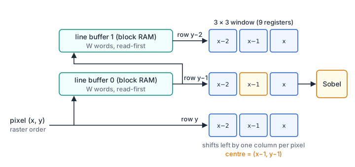
window3x3.sv
Border handling
At the edges of the image, part of the window lies outside the picture. In this design the window then contains pixels from the end of the previous line, or from the previous frame in the line buffers. The result there is meaningless and must be replaced. The common choices:
| Method | Border output | Cost |
|---|---|---|
| Constant | 0 for all window centres on the one-pixel border | A comparator on x and y |
| Replicate | Repeat the edge pixel into the missing positions | Multiplexers in front of the window |
| Mirror | Reflect pixels across the edge | Multiplexers and extra control |
This lesson uses the constant method. window3x3 sets win_ok low when the centre is on the border, that is when x < 2 or y < 2 for the newest column. The Sobel stage then outputs 0. The bottom row and right column of the image are also border pixels; because of the one-line, one-pixel lag, the stream never emits them, and they are 0 by definition. Replicate or mirror gives better results for filters such as a blur, where a black border would show.
The lag also means the edge image is shifted one pixel right and one line down relative to the input. A display pipeline either delays hsync, vsync and DE to match or accepts the shift.
Sobel gradients
The Sobel operator estimates the horizontal and vertical intensity gradient with two 3×3 kernels. Each takes a difference across the centre in one direction and smooths with weights 1, 2, 1 in the other:
Here * means: multiply each window pixel by the kernel entry in the same position and add. Gx is right minus left, Gy is bottom minus top. These are the same gradients that scipy.ndimage.sobel computes along axis 1 and axis 0; test_sobel_model.py confirms that on a test image.
The true gradient magnitude is √(Gx² + Gy²). A square root costs a lot of logic, so streaming designs often use |Gx| + |Gy|, which needs only two absolute values and an adder. It equals the true magnitude for horizontal and vertical edges and overestimates it by up to √2, a factor of 1.41, for diagonal edges. For edge detection with a threshold that is usually acceptable.
The weights 2 are shifts. With 8-bit pixels each gradient lies between -1020 and +1020, so 12-bit signed arithmetic is enough. The sum |Gx| + |Gy| is at most 1530: the two gradients cannot both be at their maximum in the same window. The function is convex in the pixel values, so its maximum lies at a window of only 0s and 255s, and test_sobel_model.py checks all 512 of them.
sobel.sv has two pipeline stages:
// Stage 1: the two gradients.
gx <= (px(win[0][2]) + 2 * px(win[1][2]) + px(win[2][2]))
    - (px(win[0][0]) + 2 * px(win[1][0]) + px(win[2][0]));
gy <= (px(win[2][0]) + 2 * px(win[2][1]) + px(win[2][2]))
    - (px(win[0][0]) + 2 * px(win[0][1]) + px(win[0][2]));
...
// Stage 2: |Gx| + |Gy|, scaling and threshold.
mag      <= ok1 ? sum[10:3] : 8'd0;
edge_out <= ok1 && (sum >= 12'(THRESH));
mag is the sum divided by 8, at most 191, so it fits in 8 bits without saturation and can be displayed directly. edge_out compares the full sum with the threshold, 400 by default. A step from black to white across a vertical edge gives |Gx| = 4 × 255 = 1020 in the pixels next to the step.
sobel.sv
Download sobel_pipeline.sv
Latency, throughput and resources
sobel_pipeline.sv chains the three blocks. Its timing:
- Throughput: one pixel per clock. With the pixel clock of lesson 19, it keeps up with 640 × 480 at 25.175 MHz or 1280 × 720 at 74.25 MHz, as long as the pipeline meets timing at that frequency.
- Latency: 6 clocks from an input pixel to its output (1 for grayscale, 3 for the window, 2 for Sobel). The result for a given pixel appears when the pixel one line and one column later arrives, so the total delay is one line plus one pixel plus 6 clocks. At 640 × 480 with blanking, one line is 800 clocks.
- Memory: two line buffers of W × 8 bits. Doubling the line length doubles them; it does not change the logic. For 1280-pixel lines each buffer is 10 240 bits.
- Logic: nine 8-bit window registers, three constant multipliers for grayscale, about a dozen adders and subtractors for the gradients, two absolute values, a comparator, and the column and row counters. No general multipliers.
The critical path is likely the gradient stage: four additions and a subtraction of 12-bit values. If it limits the clock, split it into two stages, for example the column sums first. Lesson 11 on timing analysis shows how to find and pipeline such paths.
Verifying against NumPy
sobel_model.py is the reference. It computes grayscale with the same integer formula, |Gx| + |Gy| with zero on the border, and the shifted output stream the RTL produces. test_sobel_model.py checks it against scipy.ndimage.correlate and scipy.ndimage.sobel on the interior, and checks the grayscale weights and the 1530 bound.
cocotb_sobel.py streams two synthetic 32 × 20 RGB images back to back. Each clock has a 25 % chance of being idle, with garbage on the red input, so the test exercises the valid gaps. The images come from a seeded generator: a colour gradient, a disc, a rectangle, a diagonal line and Gaussian noise, so no photograph is needed. The test checks that 640 input pixels give 640 output pixels per frame, that out_sof appears at output 0 and 640, and that every mag and edge_out value equals the model.
cd streaming-image-processing
python -m pytest -q
# 5 passed
The test catches real errors. Feeding the current row into the middle of the window instead of the line-buffer output fails at row 2, removing the rounding constant in the grayscale stage fails at the first interior pixel that rounds differently, and accepting x = 1 as an interior column fails on the first frame.
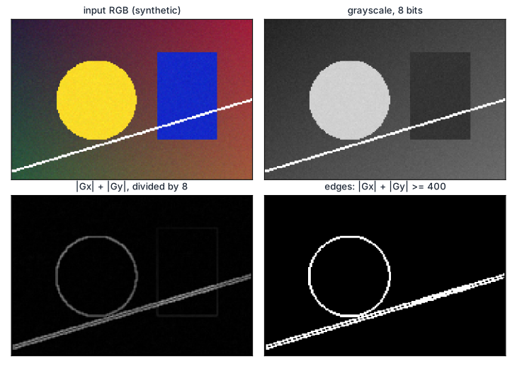
The figure comes from the NumPy model on a larger 192 × 128 image. The model matches the RTL bit for bit on the cocotb test images.
Downloadsobel_model.py
Download test_sobel_model.py
Download cocotb_sobel.py
Download test_cocotb_sobel.py
How wrong is |Gx| + |Gy|?
An edge has gradient (Gx, Gy) = (200, 0) in one place and (141, 141) in another, both with a true magnitude of about 200.
- What does |Gx| + |Gy| give in each case?
- With a threshold of 250, which edge is detected?
- Name an approximation that is closer to the true magnitude and still avoids a square root.
Show solution
- 200 for the horizontal-gradient edge, 282 for the diagonal one. The true magnitudes are 200 and √(2 × 141²) = 199.4.
- Only the diagonal edge, although both edges are equally strong. The approximation favours diagonal edges by up to a factor of √2.
- max(|Gx|, |Gy|) + min(|Gx|, |Gy|) / 2 gives 200 and 211.5 here, an error of 6 % instead of 41 % for the diagonal. It needs a comparator, a shift and an adder. The exact magnitude can also be computed with the CORDIC from FIR filters and CORDIC, at the cost of more pipeline stages.
Scale the pipeline to 1280 × 720
You want to run the edge detector on the 1280 × 720 at 60 Hz output of lesson 19.
- Which parameters change, and how much line-buffer memory is needed?
- What clock frequency must the pipeline reach?
- How long is the delay from an input pixel to its result, in clocks and in microseconds?
Show solution
- Set
W = 1280andH = 720. The column counter grows to$clog2(1280)= 11 bits and the row counter to 10 bits. The two line buffers hold 2 × 1280 × 8 = 20 480 bits. - The pixel clock, 74.25 MHz, because the pipeline takes one pixel per clock.
- One line of 1650 clocks (including blanking), plus one pixel and the 6-clock pipeline: 1657 clocks, or 1657 / 74.25 MHz = 22.3 µs.
Summary
- A streaming pipeline handles point and small-neighbourhood operations one pixel per clock with a few lines of memory; a 640 × 480 RGB frame buffer would need 7.37 Mbit.
- Grayscale with weights 77, 150 and 29 plus 128 for rounding stays within 0.945 of the BT.601 formula and maps white to 255.
- Two read-first line buffers in block RAM, one running a clock behind the other, plus nine registers form the 3 × 3 window, centred one line and one pixel behind the input.
- Sobel with |Gx| + |Gy| needs only adders; for 8-bit pixels the sum is at most 1530. Border windows output 0 in this design.
- A cocotb test with random valid gaps compares every output pixel with a NumPy model that SciPy cross-checks.
Check your understanding
Pick an answer for each question, then check. Answers stay hidden until you submit.
Further reading
- Book
- Standard
- Tool
Found a mistake or something unclear?Report a correction.
Follow this course
Get an email when new lessons and projects are added to this course.