Deployment · Lesson 12 of 12
Deployment, edge inference, FPGAs and robot safety
Budget control-loop latency, time a servo bus, quantise a model to INT8, pick an edge target, and add software and hardware safety limits to a learned policy.
What you will learn
- Build a latency budget for a camera-to-servo control loop and separate latency from throughput
- Calculate the bus time of a Sync Write and Sync Read for six Feetech servos from the packet format
- Quantise a layer to INT8 with scale and zero point, accumulate in int32, and measure the error
- Choose between an embedded GPU and an FPGA SoC, and name the jobs where an FPGA earns its place
- Add joint, speed, workspace and watchdog limits to a policy, and explain why independent hardware limits are still needed
Before you start
- Actuators and control (lesson 5)
- Sim-to-real transfer and VLAs (lesson 11)
- Optional: the FPGA course for the FPGA sections
After this lesson you can work out where the time goes between a camera frame and a servo command, compute the servo-bus share from the protocol, and shrink the inference share by quantising a model to INT8. You will know when an embedded GPU is the right target and when an FPGA is. The second half covers safety: a software filter that clamps or stops commands, a watchdog, and why the limits that really protect people must be independent of the policy computer.
The latency budget of a control loop
A learned policy on the SO-101 runs a loop: capture camera frames, preprocess, run the network, check the command, send it over the servo bus. Two numbers describe the loop, and they are not the same:
- Latency: time from the moment the scene is captured to the moment the servos receive the command based on it.
- Throughput: how often a new command goes out, the control rate.
Pipelining raises throughput by overlapping stages: capture frame while the network runs on frame . Nothing reduces latency except making the stages faster. The figure shows a budget with example values. Only the servo-bus row is computed, in the next section.
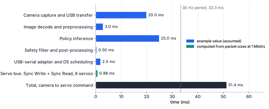
The total, 51.4 ms, is longer than the 33.3 ms period. A pipelined loop can still issue a command every 33.3 ms, but each command acts on a scene that is about 51 ms old. If the gripper moves at an example 0.3 m/s, it travels mm in that time. Three consequences follow:
- Train with the latency you deploy with. A policy trained on data where the action matched the current frame sees a different system at run time. This is the latency part of the reality gap.
- Inference is usually the biggest controllable item. Quantisation and a better target attack it directly.
- Action chunks hide throughput limits, not staleness. A policy that predicts 50 future actions can keep the arm moving while the next chunk is computed. The first action of each chunk is still based on an old frame.
Measure, do not estimate. Timestamp each stage with a monotonic clock, log every step, and report the median and the 99th percentile. A loop that averages 51 ms but takes 120 ms once a second has a 120 ms problem.
Servo-bus timing
The SO-101 drives six Feetech STS3215 servos on one half-duplex serial line. LeRobot opens the bus at 1,000,000 baud by default, and its driver backend (the rustypot library) implements the packet format. Every instruction packet looks like this:
| Bytes | Field |
|---|---|
| 2 | Header 0xFF 0xFF |
| 1 | ID (0xFE = broadcast) |
| 1 | LENGTH = number of parameters + 2 |
| 1 | Instruction: 0x83 Sync Write, 0x82 Sync Read |
| N | Parameters |
| 1 | Checksum: bitwise NOT of the low byte of the sum of ID, LENGTH, instruction and parameters |
A Sync Write of an -byte register to servos has the parameters: start address, , then for each servo its ID and data bytes. The packet is bytes. Nobody answers, so a lost packet goes unnoticed. That is the price of its speed. A Sync Read request carries address, length and the IDs, bytes. Each servo then answers with its own status packet of header, ID, LENGTH, an error byte, data bytes and a checksum: bytes.
Goal_Position (register 42) and Present_Position (register 56) are 2 bytes each on the STS3215. With UART 8N1 framing, each byte takes 10 bits, which is 10 µs at 1 Mbit/s:
| Transfer | Bytes | Time at 1 Mbit/s |
|---|---|---|
| Sync Write, 6 goal positions | 260 µs | |
| Sync Read request | 140 µs | |
| 6 status replies | 480 µs | |
| Total | 88 | 880 µs |
Each servo also waits its return delay time before answering. LeRobot writes 0 to that register as part of its recommended settings. The servos leave the factory at 250 units of 2 µs, which is 500 µs. If each of the six replies waits that long, the read grows by 3 ms. The model also leaves out the gaps between packets, the USB-to-serial adapter and operating-system scheduling. LeRobot’s driver sets its reply timeout longer than the 16 ms latency timer that a USB serial adapter can have. That is a sign that the adapter, not the wire, often dominates. The bus itself would allow over 1 kHz.
Downloadbus_timing.py
Download test_bus_timing.py
bus_timing.py builds the packets byte for byte. Its tests compare them with the Sync Read and Sync Write test vectors in rustypot’s own unit tests, checksums included.
A slower bus
Repeat the six-servo calculation at 500 kbit/s. Then add the factory return delay of 500 µs per reply. What is the highest loop rate the bus alone would allow in each case?
Show solution
The byte counts do not change: 26 + 14 + 48 = 88 bytes. At 500 kbit/s each byte takes 20 µs, so the cycle is 1760 µs and the bus alone allows about 568 Hz. With 6 × 500 µs of return delay the cycle is 4760 µs, about 210 Hz. Both are far above a 30 Hz camera loop. The bus becomes the limit only with many more servos, longer reads, or a high-rate inner loop. In practice USB adapter latency usually matters more than either figure, so measure the round trip on your own setup.
Quantisation to INT8
Most networks train in 32-bit floating point. Inference works almost as well with 8-bit integers, which need a quarter of the memory and bandwidth and run on integer multiply-accumulate (MAC) units. The common scheme is affine quantisation. A real value maps to an integer through a scale and a zero point :
For a calibrated range , widened if needed so that it contains 0:
With this choice, 0.0 maps exactly to , which matters for zero padding and ReLU outputs. Inside the range, the rounding error is at most . Outside it, values saturate. Weights are usually quantised symmetrically, with and , often with one scale per output channel. NVIDIA’s TensorRT documentation states that it uses a symmetric scheme for both activations and weights.
Worked example. Activations range from to . Then and . For : , which rounds to 32, so . Back in floating point, . The error is 0.00196, below .
Integer matrix multiply
A layer computes . Substitute the quantised forms:
Each product fits in 16 bits, because and . The sum goes into a 32-bit accumulator, which stays exact for up to about 66,000 terms. The bias is stored as int32 with scale so that it adds straight into the accumulator. One multiply by per output then converts back. On integer hardware that rescale is itself a fixed-point multiply and shift.
Downloadquantize.py
Download test_quantize.py
quantize.py quantises a 128-input, 64-output layer with random weights and runs 256 input vectors through it:
range [-1, 3]: scale = 0.015686, zero point = -64
x = 0.5 -> q = -32 -> x_hat = 0.50196
per-channel=False: max |error| = 0.1228, relative RMS error = 0.88%
per-channel=True : max |error| = 0.1003, relative RMS error = 0.69%
The tests confirm three things. The integer path equals a floating-point product of the dequantised values to within , so all error comes from rounding the inputs. The worst-case accumulator does not overflow. The layer error stays under 2 %. Errors add up through a deep network, so check the accuracy of the whole quantised model on held-out data. For a policy, that means task success on the robot, not only a loss value. If accuracy drops, calibrate the activation ranges on real data, keep sensitive layers in higher precision, or use quantisation-aware training.
Quantise by hand
A ReLU6 layer outputs values in . Find and , quantise , and give the round-trip error. Then quantise the weight symmetrically, given .
Show solution
and . Then , which rounds to 106, so . Back: , an error of , within .
For the weight, . Then , which rounds to , and .
Edge targets
Embedded GPUs such as NVIDIA’s Jetson modules run the same CUDA software as a workstation. The JetPack SDK bundles CUDA, cuDNN and the TensorRT inference runtime with Jetson Linux, and the current JetPack 7 supports the Jetson Orin and Thor platforms. A PyTorch policy can usually be exported and run with INT8 or FP16 kernels without new code. That flexibility makes an embedded GPU the default for running a policy on the robot.
FPGA SoCs put Arm processor cores and FPGA fabric on one chip. The processor runs Linux and the high-level software. The fabric holds custom logic with fixed, cycle-exact timing. Neural-network inference on an FPGA needs either a vendor accelerator IP with its compiler, or a hand-built datapath. Either way, it suits fixed, small networks better than models that change every week.
Where an FPGA earns its place
An FPGA rarely beats a GPU on raw throughput for a large model. It earns its place where timing must be guaranteed or a function must be independent of the main computer:
- Deterministic servo-bus master. A UART in fabric can send the Sync Write at an exact period, switch the half-duplex line direction within a bit time, and time-stamp every reply. No operating system or USB adapter sits in the path. The FPGA UART project builds the transmitter and receiver, and a state machine sequences the packets.
- Independent hardware safety monitor. The same logic that sees every outgoing goal position can compare it with joint limits held in fabric registers. It can block out-of-range commands and drop an enable line when a heartbeat from the processor stops. The checks run in a few clock cycles, whatever the software is doing.
- Low-latency CNN inference. A small INT8 network for a fixed task, such as a detector on a cropped image, maps onto DSP-block MACs with int32 accumulators, exactly the arithmetic above. See memory and DSP for MACs and fixed-point arithmetic in fabric.
A monitor in fabric is more independent than one in the policy process. It is still not a certified safety function by itself, and the next section explains what that takes.
Safety
A learned policy can output a command that nobody tested, in a state nobody recorded. Safety work starts from that assumption.
Risk assessment. List the hazards: pinching between links, impact, a dropped object, a cable caught in the arm. For each, estimate how severe the harm is and how likely, then reduce the risk in this order: by design (low speed, low force, rounded parts, a light arm), by safeguards (limits, fences, sensors), and last by information (labels, training). The SO-101’s small servos limit how much harm the arm can do. Larger arms raise the stakes.
Speed and separation. Keep the robot far enough from people that it can stop before contact. The required distance grows with robot speed, stopping time and how fast a person can approach.
Force limits. If contact is allowed, limit the force and pressure the robot can apply. On a servo arm that means torque and current limits in the servos and slow motion near people. The STS3215 control table has registers for a torque limit and for current protection.
Emergency stop. A hard-wired e-stop removes actuator power without going through software. For a bus-servo arm that is a switch or contactor in the servo supply, not a “stop” message on the bus.
Watchdogs. If commands stop arriving, the robot must stop and not keep executing the last chunk. A watchdog timer stops the arm when it is not fed in time.
Software limits versus independent hardware limits. Software limits are cheap, precise and easy to change, which is also their weakness: they share the computer, operating system and code base with the policy they guard. Independent limits (the angle and torque limits stored in each servo, a separate monitor, mechanical stops, the e-stop circuit) still work when the main software fails. Use both, and never rely on the policy to limit itself.
A software safety filter
safety_monitor.py sits between the policy and the bus. Each control period it checks, in order: the watchdog, the command format (shape, NaN, infinity), joint limits (clamp), speed limit (clamp the step to ), and the workspace box (forward kinematics of the clamped command must stay inside, or stop). A stop is latched. The arm holds its measured position until an operator calls reset(), because a robot that restarts by itself after a fault is a hazard.
safety_monitor.py
Download test_safety_monitor.py
The demo uses a planar two-link arm, a 20 ms period, a 2 rad/s speed limit, a workspace box with m and a 0.1 s watchdog, all example values:
Scenario 1: limits and workspace
t      command       output        status
0.00   [0.  0.5]     [0.  0.5]     ok
0.02   [0.3 0.5]     [0.04 0.5 ]   clamped
0.04   [0.1 3. ]     [0.08 0.54]   clamped
0.06   [1.  0.5]     [0.12 0.5 ]   clamped
0.08   [1.  0.5]     [0.16 0.5 ]   clamped
0.10   [1.  0.5]     [0.16 0.5 ]   stop: workspace
0.12   [1.  0.5]     [0.16 0.5 ]   stop: workspace
Scenario 2: commands stop arriving
t      command       output        status
0.00   [0.  0.5]     [0.  0.5]     ok
0.02   none          [0.  0.5]     ok
...
0.10   none          [0.  0.5]     ok
0.12   none          [0.  0.5]     stop: watchdog
A jump of 0.3 rad is cut to 0.04 rad per period, which is 2 rad/s. The request for 3.0 rad on joint 2 is clamped twice, by the 2.0 rad joint limit and then by the speed limit. When the next step would leave the box, the filter stops instead of letting the arm cross. In scenario 2 the filter repeats the last command while it is younger than the timeout, then stops. The tests also check that a late command does not clear a watchdog stop and that the arm cannot move before its first command.
The standards landscape
For industrial robots, the reference standards are ISO 10218-1:2025 (Robotics, safety requirements, Part 1: industrial robots), which covers the robot itself, and ISO 10218-2:2025 (Part 2: industrial robot applications and robot cells), which covers integrating the robot into a cell. ISO 10218-1:2025 replaced the 2011 edition of Part 1. Collaborative operation, where people and robots share a workspace, is covered further by the technical specification ISO/TS 15066:2016 (Robots and robotic devices, collaborative robots), which ISO lists as due for revision. These documents are sold by ISO and national standards bodies. A desktop arm in a lab is not automatically in their scope. Their method still applies: assess risk, reduce it by design first, and make safety functions independent of the control software. Treat this section as orientation, not compliance advice.
Logging and reporting
A deployed policy needs a record that lets someone else judge it. Log one line per control step and one per trial:
- Per step: timestamps for each stage, the raw policy output, the filtered command, the measured joint positions and the filter status.
- Per trial: success or failure, failure mode (missed grasp, dropped object, collision, timeout, safety stop), duration and the test condition.
- Per run: model and dataset versions, quantisation settings, hardware, software versions and the safety configuration.
Report success as counts with a confidence interval (see evaluating generalisation). Report latency as median and 99th percentile per stage, and failure modes as a table of counts. Count safety-filter interventions too. A policy whose commands are clamped on a large share of steps is not the policy you trained, even if the task succeeds.
Summary
- Separate latency from throughput. Pipelining keeps the control rate, but only faster stages reduce how old the observation is when the arm acts. Measure each stage and report the median and 99th percentile.
- A six-servo Sync Write plus Sync Read of 2-byte positions is 88 bytes, 880 µs at 1 Mbit/s. The factory return delay, the USB adapter and the operating system can add more than the wire time.
- INT8 affine quantisation uses with int32 accumulation. On the example layer it adds under 1 % relative error, and per-channel weight scales reduce it further.
- Embedded GPUs are the flexible default for policy inference. FPGAs earn their place as deterministic bus masters, independent safety monitors and low-latency engines for small fixed networks.
- Layer the safety: risk assessment, speed and force limits, a latched software filter with a watchdog, and independent hardware limits and a hard-wired e-stop that do not depend on the policy computer.
- Log every step and trial, and report success with intervals, latency percentiles, failure modes and safety interventions.
Check your understanding
Pick an answer for each question, then check. Answers stay hidden until you submit.
Further reading
- Paper
- Documentation
- Documentation
- Tool
Found a mistake or something unclear?Report a correction.
Follow this course
Get an email when new lessons and projects are added to this course.