Perception · Lesson 6 of 12
Camera geometry for robots: pinhole model and calibration
Project 3D points with the pinhole model, correct lens distortion, calibrate a camera, and turn a pixel into a table position for a robot arm with homographies.
What you will learn
- Project a 3D point to a pixel with the intrinsic matrix K and the extrinsics R and t
- Describe radial and tangential lens distortion and how calibration estimates it
- Explain how a checkerboard calibration recovers K from plane homographies
- Back-project a pixel to a ray and intersect it with the table plane to locate an object
- Estimate a homography with the normalised DLT and use it to map pixels to table coordinates
Before you start
- Spatial maths: rotations and homogeneous transforms (lesson 2)
- Least squares and the singular value decomposition
After this lesson you can take a pixel where a camera sees an object and turn it into a position the robot can reach. You will project 3D points with the pinhole model, know what calibration estimates and why, and use homographies to map between an image and the table the robot works on.
The pinhole model
An ideal camera maps every 3D point along a straight ray through one point, the camera centre , onto an image plane. Put the camera frame at with along the optical axis, to the right and down in the image. A point in this frame lands on the image plane at distance where, by similar triangles,
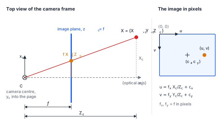
Division by is what makes the image perspective: an object twice as far away appears half as large. It also throws away depth. Every point on the ray projects to the same pixel.
The intrinsic matrix K
Pixels are counted from the top-left corner of the sensor, not from the optical axis, and they have a physical size. The intrinsic matrix collects the conversion:
The symbol means “equal up to scale”: compute the right side, then divide by its third entry, which is .
- , : focal length in pixels, the physical focal length divided by the pixel pitch. As an example, a 4 mm lens on a sensor with 3 µm pixels gives px. They differ only if the pixels are not square.
- , : the principal point, where the optical axis meets the sensor. It is near the image centre but rarely exactly on it.
- : skew, zero for practically every modern sensor.
Extrinsics R and t
Points usually come in a world or robot-base frame. The extrinsics move them into the camera frame:
and are the rotation and translation from spatial maths, in the direction world to camera. The camera centre in world coordinates is . The 3×4 matrix is the camera matrix.
Worked example
Example values for a 640 × 480 camera: px, , .
A point at m in the camera frame projects to
Now mount the camera 0.6 m above the table, looking straight down. With the world frame on the table ( up), the camera’s points along world , along world , and along world :
A point on the table at m has and projects to the same pixel, .
def project(K, R, t, X_w, dist=None):
    X_c = X_w @ R.T + t                 # world -> camera, one point per row
    z = X_c[:, 2]                       # depth; z <= 0 means behind the camera
    xn = X_c[:, :2] / z[:, None]        # normalised image coordinates
    if dist is not None:
        xn = distort(xn, dist)          # lens model, next section
    uv = xn @ K[:2, :2].T + K[:2, 2]
    return uv, z
Return the depth with the pixels. A point behind the camera still produces a pixel after the division, and only the sign of tells you it is not real.
Lens distortion
Real lenses bend straight lines, most visibly near the image edges. The usual model is the Brown-Conrady model, applied to normalised coordinates , before :
The terms are radial distortion: the image is stretched or compressed with distance from the centre. Negative gives barrel distortion (straight lines bow outwards). The terms are tangential distortion, caused by a lens that is slightly tilted relative to the sensor. The coefficient order in the download matches the order OpenCV uses.
The size is easy to underestimate. With , a point at (400 px from the centre when px) moves inwards by 5 %, which is 20 px. At 0.6 m that is about 15 mm on the table. Distortion must be removed before any of the geometry below gives millimetre accuracy.
The model maps undistorted to distorted coordinates. Going back, which you need for every measured pixel, has no closed form. undistort_normalized uses a fixed-point iteration. With and points out to , five iterations reach an error of and ten reach in normalised units.
Camera calibration
Calibration estimates and the distortion coefficients, and as a by-product the pose of the calibration target in every image. The standard method for a single camera is Zhang’s method with a flat checkerboard.
One view gives a homography
Put the world frame on the board, so every corner has . The projection then drops the third column of :
The 3×3 matrix is a homography, a projective map from one plane to another. It can be estimated from the detected corners alone (see the DLT below).
Several views give K
The columns of are , , for some scale . Because and are orthonormal, each view gives two equations on the symmetric matrix :
has six entries and is known only up to scale, so it has five unknowns, and three views in different orientations determine it. Stacking the equations gives a homogeneous system , solved with the SVD. then follows from ; the download uses a Cholesky factorisation of for this step. The download implements this linear step in intrinsics_from_homographies. On synthetic data (6 views of a 9 × 6 corner board, 0.2 px corner noise) it returns , , , px against the true 820, 810, 330 and 235.
Refinement
The linear solution ignores distortion and minimises an algebraic error rather than a geometric one. Real calibration tools use it only as a starting point. They then run a nonlinear least-squares optimisation, usually Levenberg-Marquardt, over , the distortion coefficients and one per view, minimising the reprojection error: the distance in pixels between each detected corner and where the model projects it.
The final RMS reprojection error is the number to check. A common rule of thumb is to aim for less than one pixel. A large error, or one much larger in some images, points to motion blur, a board that is not flat, or a wrong corner count.
Practical rules that follow from the maths:
- Tilt the board in many directions. Fronto-parallel views all give nearly the same constraint and leave poorly determined. Zhang (2000) names parallel board positions as a degenerate configuration of the method.
- Fill the image corners in some views. Distortion is largest there, and the model cannot be estimated from points near the centre. In Zhang’s own experiment, the views in which the board covered only the centre of the image gave unreliable distortion estimates.
- Fix the focus and the resolution. Both change , and autofocus invalidates a calibration.
From a pixel to the table
A calibrated camera turns a pixel into a ray. Undistort the pixel, apply to get a direction in the camera frame, and rotate it into the world:
To locate an object you need one more fact, and for a robot on a table the table itself provides it. Intersect the ray with the plane :
For the downward camera, pixel gives and . With and the table plane , and m, the point we started from.
Now suppose the pixel is the centre of the top face of a 25 mm cube. The correct plane is m, which gives and m. Using the table plane instead would put the cube 5.6 mm too far from the point under the camera, enough to make a gripper miss a small object. Intersect with the plane the detected feature actually lies on.
def backproject_to_plane(K, R, t, uv, normal=(0.0, 0.0, 1.0), offset=0.0, dist=None):
    n = np.asarray(normal)
    c, d = pixel_to_ray(K, R, t, uv, dist)      # camera centre, unit rays (world)
    s = (offset - c @ n) / (d @ n)
    return c + s[:, None] * d
The function in the download also rejects rays parallel to the plane and planes behind the camera.
Hand-eye calibration
The ray above is in the world frame you used for and . For a robot, that frame must be the robot base, so you need the transform between camera and base. Finding it is hand-eye calibration. There are two set-ups:
- Eye-to-hand: the camera is fixed and watches the arm, a common set-up for a desktop arm such as the SO-101. You want the constant transform from camera to robot base.
- Eye-in-hand: the camera rides on the wrist. You want the constant transform from camera to gripper. The classical formulation moves the arm to several poses, observes a fixed target each time, and solves for the unknown transform , where are relative gripper motions from forward kinematics and the matching relative camera motions. Tsai and Lenz (1989) solve this with at least three arm poses: first the rotation, then the translation, each by linear least squares.
For the fixed camera there is a direct route when you can measure 3D points in both frames. Let the gripper hold a marker, move it to a dozen positions, record each position in the base frame from forward kinematics, and measure the same positions in the camera frame (with a depth camera, or from a marker of known size). The best rigid transform between the two point sets has a closed-form SVD solution, rigid_transform in the download. With 12 points and 1 mm of noise, the test recovers the rotation to 0.13° and the translation to 0.5 mm.
Homographies for planar scenes
If everything the robot picks lies on the table, you can skip the full calibration chain. Points on a plane map to the image through a homography, so a single 3×3 matrix converts table coordinates to pixels and its inverse converts pixels to table coordinates.
The direct linear transform
Each correspondence with gives two linear equations in the nine entries of , after you multiply out the division:
Stack the rows for points into and take as the right singular vector of for the smallest singular value. This minimises subject to , which removes the scale ambiguity. No three of the points may be collinear.
Normalisation
Before building , translate each point set so its centroid is at the origin and scale it so the mean distance from the origin is . Hartley (1997) proposed this normalisation for the eight-point algorithm and notes that it applies directly to estimating projective transformations between point sets. Estimate for the normalised points, then undo the two transforms: .
T1, s = normalize_points(src)                  # table points, e.g. metres
T2, d = normalize_points(dst)                  # pixels
A = build_rows(s, d)                           # 2N x 9
_, _, vt = np.linalg.svd(A)
H = np.linalg.inv(T2) @ vt[-1].reshape(3, 3) @ T1
H /= H[2, 2]
Without normalisation, the entries of mix products such as pixels times millimetres, of order , with ones, and the result depends on the units and origin you happened to choose for the table. With it, the estimate is the same whether you measure in metres from the robot base or in millimetres from a table corner. test_normalised_dlt_is_invariant_to_world_units_and_origin checks exactly that. In double precision with well-spread points the accuracy gain is often small, but the step is cheap and removes a whole class of surprises.
Calibrating the table with the robot
A practical procedure for an arm and a fixed camera:
- Move the gripper tip to six or more points spread over the work area, touching the table. Read each position from forward kinematics.
- Detect the tip (or a small marker on it) in the image at each point.
- Estimate from table coordinates to pixels.
- At run time, map each detected object pixel through to get its table position in the robot base frame.
This folds intrinsics, extrinsics and the camera-to-base transform for that one plane into a single matrix. It does not model distortion, so undistort the pixels first or keep the work area near the image centre. It is only valid for points on that plane; for objects of known height, calibrate a second plane at that height or use the ray intersection above.
The download’s worked example does this with a tilted camera 0.45 m above the table and six touched points with 0.5 px detection noise. A cube placed at m is located with an error of 0.28 mm.
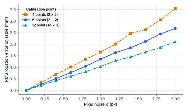
The error grows linearly with pixel noise, and more calibration points reduce it. At 0.5 px noise, four points give about 0.85 mm RMS over the work area and twelve give 0.52 mm. Spread the points to the edges of the work area: outside the calibrated region you are extrapolating and the error grows.
Code and tests
Downloadcamera.py
Download test_camera.py
python camera.py
python -m pytest -q
# 13 passed
All tests use synthetic cameras and seeded noise. They cover the worked projection, the downward-camera back-projection numbers, the project and back-project round trip with distortion, undistortion, exact homography recovery without noise, cube location with noise, invariance of the normalised DLT, Zhang’s linear calibration and the rigid transform for hand-eye calibration.
Locate a cube from one pixel
Use the downward camera from the worked example: px, , , centre 0.6 m above the table, . A detector reports the top-face centre of a 30 mm cube at pixel . Lens distortion has already been removed.
- Compute the ray direction in world coordinates.
- Find the cube’s top-face centre.
- How large is the error if you intersect with the table plane instead?
Show solution
- . (not normalised, which is fine for the intersection).
- Plane : , so m.
- Plane : , m. The horizontal error is mm, directed away from the point below the camera.
Check: backproject_to_plane(K, R, t, np.array([[200.0, 300.0]]), offset=0.03) with .
Count the constraints
- A homography has nine entries. Why do four point pairs suffice, and why does it fail if three of the four points lie on a line?
- Zhang’s linear step needs at least three views of the board. With the extra assumption that the skew is zero, how many views are enough?
- You calibrate with ten images, all taken with the board facing the camera squarely at the same distance. The reported reprojection error is low. Why can still be wrong?
Show solution
- is defined up to scale, so it has eight degrees of freedom. Each pair gives two equations (one for , one for ), and four pairs give eight. If three points are collinear, their equations are not independent. A homography maps lines to lines, so once two of the points fix where their line goes, the third point on it adds only one new equation instead of two. Four such points give seven independent equations for eight unknowns, and has a null space of more than one dimension.
- has five unknowns after removing scale. Zero skew sets , which removes one unknown, leaving four. Each view gives two equations, so two views in different orientations suffice.
- Views that all look the same give nearly identical constraints on , so the stacked system is close to rank-deficient. In particular, focal length and distance trade off against each other when the board is never tilted. The optimiser finds a that fits these images well but is wrong for other viewing angles. Low reprojection error on the calibration images does not prove a good calibration; tilted views and views that cover the image corners do.
Summary
- The pinhole model projects a world point with . holds the focal length in pixels and the principal point; and move points from the world into the camera frame.
- Lens distortion is modelled with radial () and tangential () terms on normalised coordinates. A few percent of radial distortion moves edge pixels by tens of pixels and must be removed before metric measurements.
- Zhang’s method calibrates from several views of a flat board: each view gives a homography, each homography gives two linear constraints on , and a nonlinear refinement minimises the reprojection error.
- One pixel gives only a ray. Intersecting the ray with a known plane, such as the table or the top face of an object, gives a 3D position; using the wrong plane causes a systematic error of millimetres.
- For objects on a table, a homography estimated with the normalised DLT from robot-touched points maps pixels directly to table coordinates in the robot base frame.
Check your understanding
Pick an answer for each question, then check. Answers stay hidden until you submit.
Further reading
- Paper
- Book
- Paper
- Paper
- Book
Found a mistake or something unclear?Report a correction.
Follow this course
Get an email when new lessons and projects are added to this course.