Robot learning · Lesson 10 of 12
Reinforcement learning for robots: Q-learning to PPO
MDPs and the Bellman equation, tabular Q-learning in NumPy, PPO's clipped objective, reward design for reaching, and why most robot RL runs in simulation.
What you will learn
- Write a robot task as a Markov decision process with states, actions, rewards and a discount factor
- Derive the Bellman optimality equation and solve a small MDP with value iteration
- Implement tabular Q-learning with epsilon-greedy exploration and check it against value iteration
- Explain the policy-gradient idea and the PPO clipped surrogate objective
- Design a reaching reward, spot reward hacking, and decide between RL, imitation learning or both
Before you start
- Python and NumPy
- Probability: expectations and conditional probability
- Imitation learning (lesson 8)
After this lesson you can write a robot task as a Markov decision process, solve a small one exactly with value iteration, and learn the same solution from trial and error with tabular Q-learning. You will also know how the method scales to neural networks and continuous arm commands through policy gradients and PPO, why a reaching reward is easy to get wrong, and why almost all robot reinforcement learning (RL) runs in simulation.
Learning from reward instead of demonstrations
In imitation learning the robot copies recorded actions. It can never do better than the demonstrator, and it has no signal for states the demonstrator never visited. RL replaces the demonstrations with a scalar reward that scores each step. The robot tries actions, observes the reward, and adjusts its behaviour to collect more reward over time. The upside is that RL can find behaviour nobody demonstrated. The cost is that it needs many trials, and the reward must describe the task exactly.
Markov decision processes
RL problems are written as a Markov decision process (MDP), a tuple :
- States : everything the robot needs to choose an action. For the SO-101 reaching a point, that could be the six joint angles, their velocities and the target position.
- Actions : what the policy outputs, for example six goal positions for the servos.
- Transition model : the probability of the next state. The physics of the arm defines it, and the learner usually does not know it.
- Reward : a number for each transition.
- Discount : how much a reward one step later is worth compared with now.
“Markov” means the next state depends only on the current state and action, not on the earlier history. If the robot only sees joint angles and not velocities, a fast-moving and a resting arm look the same and the Markov property fails. That is why velocities, or a short stack of past frames, often go into the state.
The agent maximises the return, the discounted sum of future rewards:
With , a reward 7 steps away is weighted by . The effective horizon is about steps. A policy maps states to (probabilities of) actions.
Value functions and the Bellman equation
The state value of a policy is its expected return from state , and the action value is the expected return after taking action in and following afterwards:
Split the return into the first reward plus the discounted rest, , and the definition becomes recursive. This is the Bellman expectation equation:
The optimal policy picks the best action in every state, which replaces the average over actions with a maximum. This is the Bellman optimality equation:
Once you have , the optimal policy is greedy: .
Value iteration turns the optimality equation into an update. Start with and apply the right-hand side to every state until nothing changes. For the update is a contraction: each sweep shrinks the largest error by at least a factor , so it converges to from any start. Value iteration needs the model , which you have for a grid world and do not have for a real arm.
A grid world as a reaching task
A 5 by 5 grid gives a discrete version of reaching. The gripper starts at S and must reach the target G. H cells are obstacles that end the episode with a penalty, and # cells are walls. Each move costs , reaching G pays , entering H pays , and moves into a wall or the edge leave the agent where it is.
S....
.##.H
...#.
.H...
...#Ggridworld.py
Download value_iteration.py
Download test_gridworld.py
Download test_value_iteration.py
value_iteration.py computes with and converges in 13 sweeps. Its greedy policy, printed as arrows, is:
v<<<<
v##^H
>>v#v
^H>>v
>>^#G
The shortest safe path takes 8 moves, so its return is seven step penalties and the goal reward. Check by hand:
which matches the program’s output of 0.9501. The top row is a trap: the route along it ends next to the hazard with a wall below, so the arrows there point back towards the start.
Tabular Q-learning
Q-learning learns without the model. After each real transition it moves a step towards a one-sample estimate of the Bellman right-hand side:
The bracket is the temporal-difference (TD) error. At a terminal state the target is just . Q-learning is off-policy: the target uses the greedy next action, so it learns the values of the greedy policy while the robot behaves with an exploring one. The inner loop of qlearning.py is short:
for t in range(max_steps):
    a = epsilon_greedy(q[s], eps, rng)
    s2, r, done = env.step(s, a, rng)
    target = r if done else r + gamma * q[s2].max()
    q[s, a] += alpha * (target - q[s, a])      # temporal-difference update
    total += r
    s = s2
    if done:
breakqlearning.py
Download test_qlearning.py
The learner only calls env.step, never env.transitions. The test file trains with 5000 episodes, and falling from 1.0 to 0.2, and checks five seeds against value iteration. Every non-terminal state must satisfy , every entry of must be within of , and every greedy action must be optimal. In a deterministic world with a constant , Q-learning converges exactly, provided every state-action pair keeps being tried. With random transitions, must decay for the estimates to settle. Run all tests from the download folder:
cd public/code/robotics-ai/reinforcement-learning
/Volumes/M2-Dev/conda/envs/toptech/bin/python -m pytest -q
Exploration
A purely greedy learner exploits whatever looks best so far and never discovers better routes. Epsilon-greedy exploration takes a uniformly random action with probability and the greedy action otherwise. With four actions and , the greedy action is chosen with probability , and each other action with . A unit test checks those frequencies.
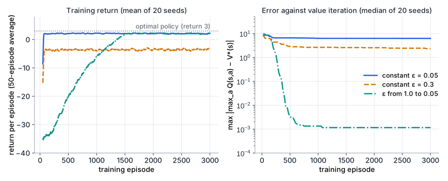
The figure shows the trade-off. With the agent finds the 8-step path within about 100 episodes. Cells away from that path, such as the bottom-left corner, are then almost never visited, and their values stay wrong by up to about 6. With the values improve, but the training return levels off near because random moves walk into hazards. The decaying schedule pays early, with returns near , and ends with both a good policy and an accurate . On a robot, every one of those early random moves is a real motion. That cost is the subject of a later section.
From tables to function approximation
A table needs one entry per state-action pair. Six joint angles discretised into 100 bins each give states before velocities are added. Real robot RL therefore replaces the table with a parameterised function , usually a neural network, and turns the update into regression on the TD target:
Here is a slowly updated copy of the weights, so the target does not move with every gradient step. Transitions are stored in a replay buffer and sampled in random minibatches to break the correlation between consecutive steps. Two difficulties appear that the table did not have. Bootstrapping from your own estimates, with a function approximator, on off-policy data can diverge. And over a continuous six-dimensional action space is itself an optimisation problem. For arm control the usual answer is to learn the policy directly.
Policy gradients and PPO
A policy-gradient method parameterises a stochastic policy , for example a Gaussian whose mean is a network output, and climbs the gradient of the expected return:
The advantage estimates how much better action was than the policy’s average in , usually as the observed return minus a learned value . Actions that did better than expected become more likely. The estimate is noisy, and one large step can wreck a policy that took hours to train.
Proximal Policy Optimization (PPO, Schulman et al., 2017) limits how far each update moves the policy. It defines the probability ratio between the new and the data-collecting policy:
and maximises the clipped surrogate objective
For a positive advantage, the objective grows with only up to . Beyond that it is flat, so there is no gradient pushing the action’s probability further. For a negative advantage, the same happens below . Taking the minimum makes the objective a pessimistic lower bound on the unclipped one. This lets PPO run several epochs of minibatch gradient steps on each batch of collected data without the policy running away. The paper uses ; in its comparison on continuous-control benchmarks, 0.2 scored better than 0.1 and 0.3. In practice the loss also includes a value-function error term and an entropy bonus, and the advantages come from generalised advantage estimation.
PPO is on-policy: data collected with is used for a few epochs and then discarded. That is simple and stable, but it needs a lot of interaction. Off-policy actor-critic methods such as Soft Actor-Critic (SAC) reuse a replay buffer and need fewer samples, which matters when the samples come from a real arm.
Reward design and reward hacking
For a reaching task with gripper position and target , three common rewards are:
- Sparse: when cm, else 0. It describes the task exactly, but random exploration almost never finds the reward in a large workspace.
- Dense: every step. It gives a gradient everywhere, but it does not say “stop” or “be gentle”.
- Shaped: the dense term plus a success bonus, minus penalties on action size , joint speed and contact force, with episode termination on success or on leaving the workspace.
The optimiser will maximise the number you give it, not the intent behind it. Reward hacking is the result. A per-step bonus for being near the target teaches the arm to hover and never finish, because touching ends the stream of reward. A reward measured on an object’s position can be collected by knocking the object towards the goal instead of grasping it. In simulation, a policy can find contact-solver errors that produce impossible forces. A missing action penalty gives jerky, bang-bang commands that wear the servos.
Two habits catch most of these. First, check the sign of the per-step reward: positive per-step rewards make survival attractive, negative ones make finishing attractive. Second, watch rollouts, not only the return curve. A rising return with strange motion is the classic symptom. Shaping that takes the form for some potential , for example , with at terminal states, adds guidance without changing which policy is optimal.
Reward hacking in the grid world
Change the step reward from to and run value iteration again (GridWorld(step_reward=1.0), ). Predict and the optimal behaviour before you run it. Then find the largest constant step reward for which reaching G is still optimal from S.
Show solution
With per step, never finishing is worth . Reaching the goal in 8 moves is worth , which is less. Value iteration returns , and the greedy policy points every cell away from G and H: the arm “reaches” forever and never arrives.
For a step reward , finishing in 8 moves is worth , and never finishing is worth . Finishing is optimal while , that is . A small positive “alive” bonus is already enough to break the task. Use a negative step reward or a zero step reward with a goal bonus.
Sample cost on real hardware
The tabular agent above used 3000 episodes and 36,673 steps (seed 0) to learn a 21-state problem. At an example rate of 10 actions per second, that is about an hour of continuous robot motion, without counting the time to reset the scene after each episode. Robot tasks have far larger, continuous state spaces, and deep RL on them needs many more steps than this toy problem.
On a real arm each step has costs that a simulator does not:
- Time: steps happen in real time, one robot at a time, and resets are slow or need a person.
- Wear and damage: random exploration hits joint limits, the table and the robot itself. Small bus servos heat up under sustained load.
- Safety: an exploring policy is by design unpredictable, so the workspace must be fenced and a person must watch.
- Reward measurement: a simulator knows the exact gripper and object positions. On the real robot, the reward has to come from cameras or a trained success classifier, which adds noise and its own failure modes.
Simulation removes most of these costs. Physics engines step faster than real time, simulated robots never wear out, and GPU-accelerated frameworks such as Isaac Lab speed up the physics further. The price is the gap between the simulated and the real robot, which the next lesson, sim-to-real transfer and VLAs, covers.
Real-robot RL is possible when the task is short and the setup limits exploration. The LeRobot documentation describes a human-in-the-loop workflow (HIL-SERL) for arms such as the SO-101. It starts from a few teleoperated demonstrations, trains a vision-based reward classifier, and runs an off-policy SAC learner while a person can take over the arm at any time. It also bounds the end-effector workspace so that exploration stays in a safe box.
RL, imitation learning, or both
| Imitation learning | Reinforcement learning | |
|---|---|---|
| Training signal | Demonstrated actions | Scalar reward |
| Data source | Teleoperation, fixed dataset | The policy’s own trials |
| Can exceed the demonstrator | No | Yes |
| Main risk | Compounding errors off the demonstrated states | Sample cost, reward hacking, unsafe exploration |
| Typical setting | Real robot, tens to hundreds of episodes | Simulation, or short real tasks with safeguards |
The two combine well:
- Pretrain, then fine-tune. Behaviour cloning gives a policy that already succeeds sometimes, and RL improves it. This avoids the hopeless random start of sparse-reward tasks.
- Demonstrations in the replay buffer. An off-policy learner can mix demonstration transitions with its own, as the HIL-SERL workflow does.
- Human interventions as data. When a person takes over, the corrected actions are recorded and the policy learns from them.
- RL in simulation as a teacher. A policy trained with privileged simulator state (exact object poses) can generate demonstrations for a camera-based student policy trained by imitation.
For a new manipulation task on the SO-101, start with imitation learning (ACT and diffusion policies) and reach for RL when you need to go beyond what the demonstrations show, or when the task is defined better by an outcome than by a motion.
One Q-learning update by hand
In the grid world with and , the agent is in the cell directly above G and all values are still 0. It moves down, enters G and receives . What is the new for that state and action? In a later episode, before the cell above G is visited again, the agent is in the cell to the left of it, moves right and receives . What is the update now, and what value does it converge to?
Show solution
G is terminal, so the target is just the reward: . Each later visit halves the gap, giving 7.5, 8.75 and so on towards 10.
For the move into the cell above G, the target is , so . As the value above G approaches 10, the target approaches . Value iteration gives the same 8.5 for that state, two steps from the goal.
Summary
- An MDP has states, actions, a transition model, a reward and a discount . The agent maximises the discounted return, with an effective horizon of about steps.
- The Bellman optimality equation defines and . Value iteration solves it when the model is known, and the greedy policy on is optimal.
- Tabular Q-learning learns from sampled transitions with the TD update. It only learns what it visits, so exploration such as decaying epsilon-greedy decides how good the values become.
- Large and continuous problems need function approximation. Policy-gradient methods such as PPO learn the policy directly, and PPO’s clipped ratio keeps each update close to the data-collecting policy.
- Reward design is the hardest part of robot RL: positive per-step rewards, measurable proxies and missing penalties all invite reward hacking, so watch the rollouts.
- Real-robot samples are slow, costly and risky, so most robot RL runs in simulation. Combining RL with demonstrations and human interventions cuts the number of real trials.
Check your understanding
Pick an answer for each question, then check. Answers stay hidden until you submit.
Further reading
- Book
- Paper
- Documentation
Found a mistake or something unclear?Report a correction.
Follow this course
Get an email when new lessons and projects are added to this course.