Kinematics and control · Lesson 4 of 12
Inverse kinematics and Jacobians for robot arms
Solve inverse kinematics for a 2-link arm in closed form, build the Jacobian, find singularities, and write damped least-squares IK and resolved-rate control.
What you will learn
- Solve the planar 2-link inverse kinematics in closed form and pick the elbow-up or elbow-down solution
- Build the Jacobian of a serial chain analytically or by finite differences and explain what its columns mean
- Detect singularities from the determinant, the manipulability and the singular values of the Jacobian
- Implement Jacobian-transpose, pseudo-inverse and damped least-squares IK and choose the damping factor
- Command Cartesian tip velocities with resolved-rate control while respecting joint limits
Before you start
- Spatial maths: rotations and homogeneous transforms (lesson 2)
- Forward kinematics (lesson 3)
- Matrix inverse and least squares from linear algebra
After this lesson you can compute the joint angles that put a robot arm’s tip at a given point, both in closed form for a 2-link arm and numerically for any serial chain. You will use the Jacobian to relate joint velocities to tip velocity, recognise singular configurations before they cause trouble, and drive the tip along a straight line with resolved-rate control.
The inverse problem
Forward kinematics maps joint angles to a tip pose . It always has exactly one answer. Inverse kinematics (IK) asks for the that gives a wanted , and that question can have no solution, a finite number of solutions or infinitely many:
- No solution: the target lies outside the workspace, or the arm lacks the joints to reach that orientation.
- A finite number: a planar 2-link arm reaches most points in two ways, elbow up and elbow down.
- Infinitely many: the arm is redundant, with more joints than task coordinates. A planar 3-link arm placing only its tip position has one spare degree of freedom.
The SO-101 follower arm has five arm joints (shoulder pan, shoulder lift, elbow flex, wrist flex, wrist roll) plus a gripper. A full pose in 3D has six numbers, so the SO-101 cannot reach an arbitrary position and orientation; a target pose must be chosen within what five joints can do. Its shoulder lift, elbow flex and wrist flex axes are parallel, so once the shoulder pan has turned the arm towards the target, the shoulder and elbow form a planar 2-link arm in a vertical plane. In the SO-101 URDF published in the SO-ARM100 repository, the elbow axis sits about 0.116 m from the shoulder-lift axis and the wrist-flex axis about 0.135 m from the elbow. That is why the planar case below is not only a textbook exercise.
Analytic IK for the planar 2-link arm
Take two links of length and , joint angles (from the x axis) and (relative to link 1). Forward kinematics is
Elbow angle from the law of cosines
The base, elbow and tip form a triangle with sides , and . The law of cosines gives the elbow angle directly:
The sign choice gives the two solutions. With the convention in the download, is called elbow down and elbow up; for a target to the right of the base, puts the elbow below the line from base to tip. Use atan2 rather than acos: it keeps the sign and stays accurate near and .
Shoulder angle
The shoulder angle is the direction to the target minus the angle that link 2 adds:
Reachability
A real exists only if , which is the same as
The workspace is an annulus. On its outer circle the arm is fully stretched () and on the inner circle fully folded (); there the two solutions merge into one. Real joint limits cut further pieces out of the annulus, so check the limits after solving.
Worked example
Example values: m, m, target m.
- , so m, inside the annulus from 0.10 m to 0.50 m.
- .
- Elbow down: , .
- and , so .
- Elbow up: and .
Always check an IK result with forward kinematics. A condensed version of ik_2link from the download:
def ik_2link(x: float, y: float, l1: float, l2: float,
             elbow: Literal["up", "down"] = "down") -> tuple[float, float]:
    r2 = x * x + y * y
    c2 = (r2 - l1 * l1 - l2 * l2) / (2.0 * l1 * l2)
    if c2 > 1.0 + 1e-12 or c2 < -1.0 - 1e-12:
        raise ValueError("target is out of reach")
    c2 = float(np.clip(c2, -1.0, 1.0))
    s2 = np.sqrt(1.0 - c2 * c2) * (1.0 if elbow == "down" else -1.0)
    q2 = np.arctan2(s2, c2)
    q1 = np.arctan2(y, x) - np.arctan2(l2 * s2, l1 + l2 * c2)
    return float(q1), float(q2)
$ python ik.py
elbow down: q1 = 1.22 deg, q2 = 74.29 deg, FK -> (0.3500, 0.2000)
elbow up : q1 = 58.27 deg, q2 = -74.29 deg, FK -> (0.3500, 0.2000)The np.clip matters: a target exactly on the boundary can give from rounding, and sqrt of a tiny negative number returns NaN.
The Jacobian
Closed-form IK exists only for simple geometries. For the general case you need the Jacobian, the matrix of partial derivatives of the forward kinematics:
Column is the tip velocity you get when joint turns at 1 rad/s and all other joints are still. For a revolute joint with unit axis through point , the tip at moves with linear velocity , and the tip frame rotates with angular velocity . Stacking both gives the 6-row geometric Jacobian of a spatial arm. When you only care about tip position, keep the top three rows.
For the planar 2-link arm every axis points out of the page, and the cross product reduces to a 90° rotation of the vector from joint to tip:
At the elbow-down solution of the worked example:
The first column is of the tip, as expected for rotation about the base. Turning joint 1 at 0.1 rad/s moves the tip at m/s.
Numerical Jacobian
If you have forward kinematics as code but no derivation, central differences give the Jacobian with error proportional to :
With rad this costs forward-kinematics calls and matches the analytic Jacobian to about . test_ik.py checks the match, to within , for a 4-link chain. It is the easy way to get a Jacobian for an arm described by a chain of transforms from lesson 3.
Singularities
For a square Jacobian you can invert the velocity relation, , as long as . For the 2-link arm,
It is zero when the arm is straight () or folded back (). In those configurations the tip cannot move along the line through the base, whatever the joints do. Close to them, a modest tip velocity needs huge joint velocities. The table holds and asks for 0.1 m/s along x, the direction of link 1, with m and m:
| Elbow angle | (m²) | Joint speed (rad/s) |
|---|---|---|
| 90° | 0.0600 | 0.50 |
| 30° | 0.0300 | 1.68 |
| 5° | 0.0052 | 10.3 |
| 1° | 0.0010 | 51.4 |
No hobby servo turns at 50 rad/s. A controller that inverts blindly near a singularity either saturates the motors or makes the arm jump.
Manipulability and singular values
For non-square Jacobians (a redundant arm, or a 5-joint arm with a 6-row Jacobian) the determinant is undefined. Two measures work for any shape:
- Manipulability . It equals for a square and is zero at a singularity. It is a convenient scalar for “how far from singular” and is often maximised with spare degrees of freedom.
- Singular values from the SVD . Each is the tip speed along that a unit joint velocity along produces. The smallest one says how weak the worst direction is, and is the condition number.
At the worked-example configuration the singular values are 0.429 and 0.134, so the arm is far from singular. At they are 0.538 and 0.0019.
Singularities are not only at the workspace boundary. A spatial arm with a spherical wrist has a wrist singularity when two wrist axes line up, which can happen in the middle of the workspace.
Numerical IK as optimisation
For a general chain, write IK as a least-squares problem:
Linearise around the current guess, , take a step, and repeat until is below a tolerance. The methods differ only in how they compute from and .
Jacobian transpose
is the negative gradient of , so this is gradient descent. It needs no matrix inverse and never blows up, but convergence along each singular direction scales with , so it is slow when the singular values differ, and too large an makes it oscillate.
Pseudo-inverse
This is the Gauss-Newton step. For a redundant arm it gives the smallest joint step that removes the linearised error. It converges in a few iterations when the arm is well away from singularities. Near one, explodes.
Damped least squares
Damped least squares (DLS), also called the Levenberg-Marquardt step, adds a penalty on the step size:
In terms of the SVD, DLS replaces with
For this is almost , so DLS behaves like the pseudo-inverse. For it is about , which goes to zero: DLS stops pushing in directions the arm cannot move. The largest gain, , occurs at , so a single step can never exceed .
The price is accuracy. With a step does not remove the full linearised error, so the solver needs more iterations, and in resolved-rate control the tip lags the commanded velocity. A common choice is a little below the smallest singular value you expect in normal operation, in the same units as (metres per radian here). Some implementations raise only when or drops below a threshold.
The core of ik_solve in the download:
for k in range(max_iter):
    err = target - fk(q)
    if np.linalg.norm(err) < tol:
        break
    jmat = jac_fn(q)                       # analytic, or central differences
    if method == "transpose":
        dq = alpha * jmat.T @ err
    elif method == "pinv":
        dq = np.linalg.pinv(jmat) @ err
    else:                                  # "dls"
        dq = jmat.T @ np.linalg.solve(jmat @ jmat.T + lam**2 * np.eye(len(err)), err)
    q = np.clip(q + dq, q_min, q_max)      # joint limits
Use np.linalg.solve rather than forming an inverse. is (2×2 or 6×6), so the solve is cheap even for a long chain.
Comparing the three methods
The figure runs all three methods from the same start, rad, on the 0.30 m / 0.20 m arm.
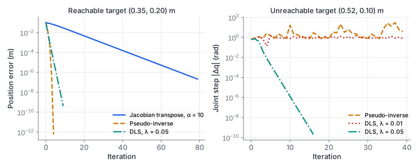
On the reachable target the pseudo-inverse converges to below 1 µm in 3 iterations, DLS with in 6, and the transpose method in 70.
The unreachable target is where the methods separate. The best the arm can do is to stretch out and point at the target, which is exactly the singular configuration. The pseudo-inverse keeps trying to remove an error it cannot remove; its steps reach 30 rad and the joints spin. DLS with settles at the straight arm pointing at the target, 0.0295 m short, which is the closest reachable point. With the damping is too weak for this case and the steps stay near 1 rad. In a real arm you would also cap the step size (max_step in the download) and report that the target is out of reach.
Joint limits
Every real joint has limits, and the SO-101 servos store a minimum and maximum position limit in their own registers. Three ways to respect limits in numerical IK, in order of effort:
- Clip to the limits after each step, as
ik_solvedoes. Simple and often enough. It can stall when the solution needs a joint to stay at its limit while others move, because the clipped joint keeps asking for the same step. - Remove a joint from the problem once it sits at a limit (set its Jacobian column to zero) and solve with the rest.
- Add a cost that grows near the limits, or use a constrained solver such as a small quadratic program per step.
For a redundant arm there is a fourth option: use the spare degrees of freedom, through the null space of , to move joints away from their limits without moving the tip.
Resolved-rate control
The same linearisation gives a velocity controller. To move the tip with velocity , command
where is the pseudo-inverse or the DLS inverse. This is resolved-rate control: the Cartesian rate is resolved into joint rates at every control period. Drawing a straight line, inserting a peg or following a camera target all use it.
Two details make it work on hardware:
- Close the loop on position. Integrating drifts, because the linearisation is only exact for an infinitesimal step. Add a correction towards the desired tip position: .
- Send positions to position-controlled servos. Bus servos such as the SO-101’s STS3215 run their own position loop, so the usual pattern is to compute in Python and write it as the goal position at a fixed rate. Actuators, joint control and trajectories covers what happens inside the servo.
In the download, resolved_rate_step performs one step. The test moves the tip of the 2-link arm 0.1 m upwards at 0.1 m/s with a 2 ms period, and the tip ends 0.03 mm from the straight-line target without any position correction (the test allows 2 mm).
ik.py
Download test_ik.py
python ik.py
python -m pytest -q
# 16 passed
The tests cover FK(IK(x)) = x for 200 random targets per elbow branch, the analytic Jacobian against finite differences, DLS with a finite-difference Jacobian on a 3-joint spatial arm (base yaw, shoulder pitch, elbow pitch), the bounded DLS step at an exact singularity, joint limits, and the pseudo-inverse blow-up on the unreachable target.
Both IK solutions by hand
Use m and m.
- Is the target m reachable?
- Compute and in degrees for both elbow solutions.
- Compute for the elbow-down solution. Is it closer to or further from a singularity than the worked example?
Show solution
- m, which is between 0.10 m and 0.50 m. Reachable.
- , so and . and . Elbow down: , . Elbow up: , .
- m². The worked example had 0.0578 m², so both are close to the maximum of 0.06 m² at and far from singular.
Check: ik_2link(0.10, 0.40, 0.30, 0.20, "down") returns (48.75°, 70.53°) after conversion to degrees.
Choose the damping factor
A resolved-rate controller uses DLS. The largest tip error it ever sees in one control period is 5 mm, and you want no single step to move a joint by more than 0.05 rad.
- Using the bound on the DLS gain, find the smallest that guarantees this.
- In normal operation the smallest singular value of your arm’s position Jacobian is about 0.10 m/rad. What fraction of the commanded motion along that direction does one DLS step achieve with your ?
Show solution
- The step is at most . Require , so m/rad.
- Along a direction with singular value , DLS achieves of the requested motion. With and : . One step removes 80 % of the error in that direction, and the next steps remove most of the rest. If that lag is too large, use a smaller away from singularities and raise it only when falls, together with a step cap.
Summary
- The planar 2-link arm has a closed-form IK: the law of cosines gives (two signs for elbow up and down), and follows from two
atan2calls. The workspace is the annulus . - The Jacobian maps joint velocities to tip velocity. Each column is the tip velocity from one joint; build it analytically or with central differences.
- Singularities are configurations where the Jacobian loses rank. , the manipulability and the smallest singular value all measure how close you are, and joint speeds grow as near them.
- Numerical IK minimises the squared tip error. The transpose method is gradient descent, the pseudo-inverse is Gauss-Newton, and damped least squares bounds every step by at the cost of slower convergence.
- Resolved-rate control applies the same inverse to velocities every control period, with a position correction and, on servo arms, goal positions sent at a fixed rate.
Check your understanding
Pick an answer for each question, then check. Answers stay hidden until you submit.
Further reading
- Book
- Book
- Article
- Paper
- Paper
Found a mistake or something unclear?Report a correction.
Follow this course
Get an email when new lessons and projects are added to this course.