Kinematics and control · Lesson 5 of 12
Actuators, PID joint control and trajectories
How DC motors, gearboxes and smart bus servos drive a robot joint, how to write a discrete PID controller with anti-windup, and how to plan smooth trajectories.
What you will learn
- Explain the torque-speed trade-off of a DC motor and how a gear ratio changes torque, speed and reflected inertia
- Describe what a smart bus servo controls internally and which settings you can change over the bus
- Implement a discrete PID controller with derivative on measurement, a derivative filter and anti-windup
- Predict the step response of a joint under P and PD control from its inertia and damping, and tune the gains
- Generate cubic, quintic and trapezoidal trajectories and choose between them for a servo-driven arm
Before you start
- Inverse kinematics and Jacobians (lesson 4)
- First-year calculus: derivatives and simple differential equations
After this lesson you can explain what limits the torque and speed of a geared motor, write a discrete PID controller that behaves well under saturation and noise, and predict how a joint responds to your gains. You will also plan smooth point-to-point moves and know why a servo arm should never be sent a raw step.
DC motors and gearboxes
Most small robot joints use a DC motor and a gearbox. Two constants describe the motor. The torque constant gives torque per ampere, and the back-EMF constant gives the voltage the spinning motor generates per rad/s. In SI units the two are equal. With winding resistance and supply voltage :
Eliminating the current gives a straight torque-speed line:
At standstill the motor gives its stall torque and draws its largest current. At the no-load speed it gives no torque. Mechanical power peaks at half the no-load speed. A higher supply voltage moves the whole line outwards.
What a gear ratio does
Small motors spin fast and give little torque, while a robot joint needs the opposite. A gearbox with ratio (output turns once for every motor turns) changes three things:
| Quantity at the joint | Effect of ratio |
|---|---|
| Torque | multiplied by , times the gearbox efficiency |
| Speed | divided by |
| Motor rotor inertia seen at the joint | multiplied by |
Example values for a small motor: mN m, rad/s, rotor inertia kg m². Behind a 345:1 gearbox, and ignoring losses, the joint has a stall torque of 3.45 N m and a no-load speed of 2.9 rad/s. The reflected rotor inertia is kg m², which is larger than the inertia of a light link of a desktop arm. This is why each joint of a highly geared arm behaves roughly like an independent inertia with damping, the model used for the controller below.
The square law also explains backdrivability. Turning the output by hand has to spin the motor times faster through all the gear friction. A high ratio makes a joint hold its pose without power but hard to move by hand.
The SO-101 uses this trade-off on purpose. According to the SO-101 assembly guide in the LeRobot documentation, the follower arm uses six STS3215 servos with 1/345 gearing. The leader arm, which you move by hand during teleoperation, mixes three ratios so that it can hold its own weight yet moves without much force:
| Leader joint | Gear ratio |
|---|---|
| Shoulder pan | 1/191 |
| Shoulder lift | 1/345 |
| Elbow flex | 1/191 |
| Wrist flex, wrist roll, gripper | 1/147 |
The shoulder lift carries the most weight and keeps the highest ratio. The SO-ARM100 repository lists the 7.4 V STS3215 at a stall torque of 16.5 kg·cm at 6 V (about 1.6 N m) and a 12 V version at 30 kg·cm (about 2.9 N m).
Smart bus servos
A smart bus servo such as the Feetech STS3215 contains the motor, the gearbox, a position sensor and a microcontroller that runs the position loop. You talk to it over a shared serial bus, where each servo has an ID and a table of registers. In the STS3215 definition that LeRobot uses (from its rustypot dependency), a full turn is 4096 position steps (12 bits), and the factory baud rate is 1 Mbit/s.
The registers you are most likely to touch, with the names LeRobot uses for the STS3215:
| Register | What it sets |
|---|---|
Torque_Enable | Motor on or off. With torque off you can move the joint by hand |
Operating_Mode | 0 position, 1 velocity, 2 PWM (open loop), 3 step |
Goal_Position, Present_Position | Target and measured position, in steps |
P_Coefficient, I_Coefficient, D_Coefficient | Gains of the internal position loop |
Acceleration | Acceleration the servo uses when it moves to a new goal |
Goal_Velocity | Target speed in velocity mode |
Torque_Limit, Max_Torque_Limit | Caps on motor output |
Min_Position_Limit, Max_Position_Limit | Position range the servo accepts |
Protection_Current, Overload_Torque | Current and overload protection |
On connect, LeRobot’s SO-101 follower code puts each servo in position mode and writes P_Coefficient = 16, I_Coefficient = 0 and D_Coefficient = 32. For the gripper it also writes Max_Torque_Limit = 500, commented in the source as 50 % of the maximum torque, to avoid burning out the motor while it grips. Its general motor setup writes 254 to both Acceleration and the Maximum_Acceleration ceiling, which the source describes as high to speed up acceleration and deceleration, so smoothness has to come mostly from the goal positions you send. The gain registers hold raw integers in firmware units, not SI gains; tune them by experiment.
This snippet follows the docstring example in LeRobot’s SerialMotorsBus source. It needs LeRobot and a servo on a USB bus adapter, and it was not run for this lesson:
# LeRobot snippet, not run here. Check the current LeRobot docs for API changes.
from lerobot.motors import Motor, MotorNormMode, SerialMotorsBus

bus = SerialMotorsBus(
    port="/dev/tty.usbmodem575E0031751",          # find yours with lerobot-find-port
    motors={"my_motor": Motor(1, "sts3215", MotorNormMode.RANGE_M100_100)},
)
bus.connect()
position = bus.read("Present_Position", "my_motor", normalize=False)
bus.write("Goal_Position", "my_motor", position + 30, normalize=False)   # 30 steps, about 2.6 degrees
bus.disconnect()
A joint as a second-order system
Model one joint, motor plus link, as an inertia with viscous damping and a constant load torque (gravity at a fixed pose):
The example values used from here on are kg m², N m s/rad and, where a load is present, N m. They are of the right order for a geared desktop-arm joint but are not measured values of any servo.
P control
With and no load, the closed loop is
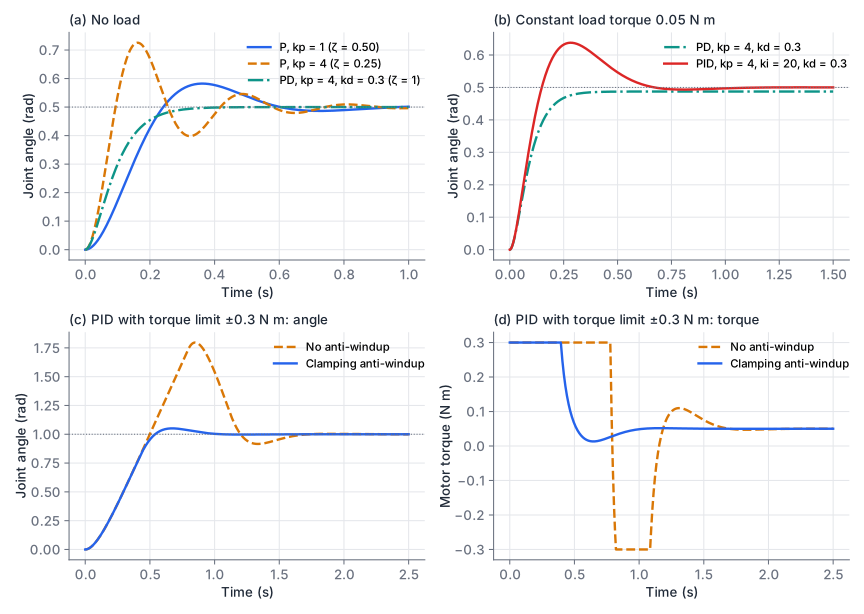
The step overshoot for is . With N m/rad, rad/s and , so the predicted overshoot is 16.3 %; the simulation gives 16.5 % (the extra comes from the 1 ms sampling). Raising to 4 doubles but halves to 0.25, and the overshoot rises to 45 %. A stiffer P controller is faster and more oscillatory.
PD control
A derivative term adds damping without changing stiffness:
For and (critical damping) you need , so N m s/rad. The step response has no overshoot and settles to within 2 % in 294 ms. The download’s pd_gains(J, b, omega_n, zeta) computes the two gains for any target.
PID control and the load offset
With a load, a PD controller settles where the spring term balances it: , so mrad. An integral term removes the offset, because the integral keeps growing as long as any error remains:
Adding N m/(rad s) removes the offset but brings back overshoot (28 % here), because the integral also builds up while the joint is still rising. The figure shows these cases.
A discrete PID controller
A controller on a microcontroller or a PC runs once every period . The download’s PID.update does this:
def update(self, setpoint: float, measurement: float) -> float:
    err = setpoint - measurement
    # derivative on measurement, low-pass filtered
    raw_d = 0.0 if self._prev_meas is None else -(measurement - self._prev_meas) / self.dt
    a = self.tau_d / (self.tau_d + self.dt) if self.tau_d > 0.0 else 0.0
    self._d_filt = a * self._d_filt + (1.0 - a) * raw_d
    self._prev_meas = measurement
    d_term = self.kd * self._d_filt
    # integral with anti-windup by clamping
    i_new = self.integral + self.ki * err * self.dt
    u_unsat = self.kp * err + i_new + d_term
    u = float(np.clip(u_unsat, self.u_min, self.u_max))
    pushing_up = u_unsat > self.u_max and err > 0.0
    pushing_down = u_unsat < self.u_min and err < 0.0
    if not (pushing_up or pushing_down):
        self.integral = i_new
    return u
(The full class also supports derivative on error, back-calculation anti-windup and a reset.) Four details matter.
The integral is stored in output units. The code accumulates , not . If you retune while the loop runs, the output does not jump.
Derivative on measurement. The derivative of the error contains the derivative of the setpoint. A step in the setpoint then produces one enormous sample: with and ms, a 1 rad step gives a 500 N m spike. Differentiating instead gives the same damping without the kick.
Derivative filter. Differencing amplifies sensor noise by . A first-order low-pass with a time constant of a few sample periods cuts the noise. In the test, 1 mrad of measurement noise with ms reduces the standard deviation of the controller output from 0.40 N m to 0.053 N m.
Anti-windup. While the output sits at its limit, a plain integrator keeps summing. When the joint reaches the target, the stored integral must unwind before the torque can reverse, so the joint overshoots far past it. Panels c and d of the figure show a 1 rad step with the torque limited to ±0.3 N m: without protection the joint overshoots by 80 % and takes 1.6 s to settle. Two standard fixes:
- Clamping (conditional integration): stop integrating while the output is saturated and the error would push it further. Overshoot drops to 5 % and settling to 0.88 s.
- Back-calculation: feed the difference between saturated and unsaturated output back into the integrator with a tracking time constant , so the integral bleeds off while saturated. It behaves similarly.
Tuning by hand
For a joint you can model, place the poles with pd_gains and add a small . Otherwise:
- With , raise until the step response overshoots clearly.
- Raise until the overshoot is gone. If the motor gets noisy or hot, filter the derivative more or lower .
- Add until the offset disappears in an acceptable time, then test a large step at the real torque limit.
- Run the loop much faster than the closed-loop bandwidth. A common rule of thumb is at least ten times faster (here about 3 Hz against 1 kHz).
Smooth trajectories
A step in the goal position asks for infinite velocity. The controller saturates and the arm jerks, which shock-loads the gears and can shake an object out of the gripper. The fix is to send a reference that moves smoothly from start to goal in a chosen time , and let the controller track it.
Cubic polynomial
A cubic has four coefficients, enough to match position and velocity at both ends. For a rest-to-rest move of :
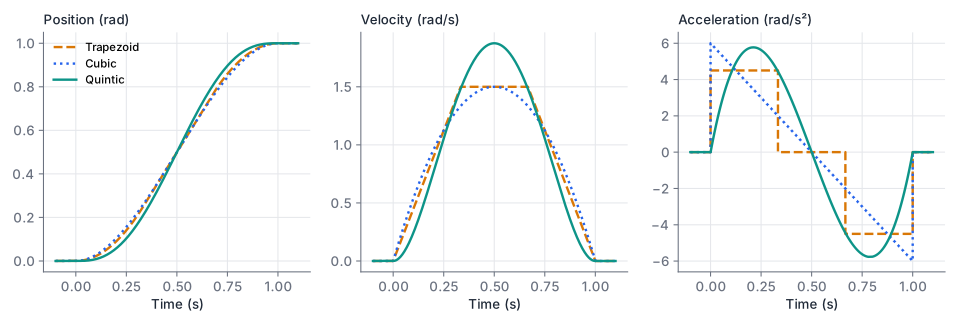
Peak velocity is at mid-move. The acceleration, however, is at and at , so it jumps at both ends. Commanded torque jumps with it.
Quintic polynomial
A quintic adds two coefficients, enough to set the acceleration at both ends as well. Rest to rest with zero end acceleration:
Peak velocity is and peak acceleration , both reached smoothly. The rest-to-rest quintic is also the minimum-jerk profile, the one that minimises the integral of squared jerk over the move. quintic_coeffs in the download solves the 6×6 linear system, so it also handles non-zero end velocities and accelerations, for example to join segments.
Trapezoidal velocity profile
Industrial drives often use a trapezoid: accelerate at , cruise at , decelerate at . For a distance :
If the move is too short to reach , the profile becomes a triangle with peak velocity . The trapezoid uses the actuator limits fully, so for given limits it is the fastest of the three. Its acceleration jumps four times, at the start and end of each ramp.
Which one for a servo arm
For a position-controlled bus servo, a quintic in joint space is a good default. It is smooth at both ends and synchronises all joints if you give them the same . Choose so that every joint stays within its limits, for velocity . Use a trapezoid when cycle time matters and the drive tolerates acceleration steps.
Send samples of the trajectory at your command rate, not the final goal; sample(profile, T, rate_hz) in the download does this. LeRobot’s follower configuration also has a max_relative_target option that caps how far a single command may move from the present position, a safety net against sending a step by mistake.
Tracking a trajectory with feedforward
A trajectory also gives the reference velocity and acceleration, so you can compute the torque the joint should need and add it to the PID output:
The PID then only corrects model errors and disturbances. One detail changes: for a smooth reference, use the derivative of the error, not of the measurement. Derivative on measurement damps the actual velocity, so it brakes the joint during the whole move. On the 0.5 rad quintic over 0.5 s with the load present, the test in the download measures a peak tracking error of 127 mrad for the plain step-tuned PID and 0.2 mrad with feedforward and derivative on error.
Learning a residual on top of a controller
In residual control, a learned policy outputs a correction that is added to a conventional controller:
The classical part, for example the PID and feedforward above, gives sensible behaviour before any training. The learned part only has to capture what the model misses, such as friction, cable forces or contact, which is a smaller problem than learning the whole controller. Bound the residual, for example to a fraction of the torque limit, so a bad network output cannot override the baseline. The approach appears under the names residual reinforcement learning and residual policy learning (see further reading). Reinforcement learning covers how such a policy is trained.
Code and tests
Downloadpid.py
Download trajectory.py
Download test_pid.py
Download test_trajectory.py
python pid.py
python trajectory.py
python -m pytest -q
# 22 passed
pid.py prints step metrics for the gain sets in the figure. The tests check the overshoot against the second-order formula, the load offset, both anti-windup methods, the derivative kick and filter, the trajectory boundary conditions and peaks, and the tracking result above.
Design a PD controller and predict its offset
The joint has kg m² and N m s/rad.
- Choose and for a critically damped response with rad/s.
- With a constant load of 0.05 N m, what steady-state error remains?
- Your torque limit is 0.5 N m. For a 0.5 rad step, does the controller saturate at the first sample? What should you do about it?
Show solution
- N m/rad. N m s/rad.
pd_gains(0.01, 0.1, 30.0, 1.0)returns (9.0, 0.5). - mrad. Raising from 20 to 30 rad/s multiplied by 2.25 and divided the offset by the same factor, but it is still there; an integral term removes it.
- Yes. The first sample asks for N m, nine times the limit. Send a trajectory instead of a step: a quintic over seconds needs a peak torque of about for the motion itself, which for s is at most N m, plus 0.05 N m for the load, so it stays below 0.5 N m.
Fit a move into the joint limits
A joint must move 1.2 rad. It may not exceed 2 rad/s or 8 rad/s².
- How long does the fastest trapezoidal move take?
- What is the shortest quintic move that respects the velocity limit? Check that it also respects the acceleration limit.
Show solution
- , so the profile reaches the cruise speed. s. s. Check with
trapezoid_duration(1.2, 2.0, 8.0), which returns (0.85, 0.25, 2.0). - Velocity: gives s. Acceleration at that : rad/s², below 8. The quintic takes 0.275 s longer than the trapezoid, the price of a smooth start and stop.
Summary
- A DC motor trades torque against speed along a straight line. A gear ratio multiplies torque by (less losses), divides speed by and multiplies the reflected rotor inertia by , which also makes the joint harder to backdrive.
- A smart bus servo such as the STS3215 runs its own position loop. Over the bus you set goal position, PID gains, acceleration, torque limits and position limits; LeRobot writes several of these registers when it connects to or calibrates an SO-101.
- Under P control a joint behaves as a second-order system with and . The D term adds damping, the I term removes the offset from constant loads.
- A good discrete PID stores the integral in output units, differentiates the measurement for step setpoints, filters the derivative, and stops the integral from winding up while the output saturates.
- Send smooth trajectories, not steps. A quintic gives zero velocity and acceleration at both ends; a trapezoid is fastest for given limits. Feedforward from the reference trajectory leaves the PID only the residual error to correct.
Check your understanding
Pick an answer for each question, then check. Answers stay hidden until you submit.
Further reading
- Book
- Book
- Paper
- Paper
- Paper
- Documentation
Found a mistake or something unclear?Report a correction.
Follow this course
Get an email when new lessons and projects are added to this course.