Deployment · Lesson 11 of 12
Sim-to-real transfer and vision-language-action models
Close the reality gap with system identification and domain randomisation, then see how VLA models such as SmolVLA map images and instructions to robot actions.
What you will learn
- Name the parts of the reality gap (dynamics, sensing, latency, visuals) and how each shows up on a servo arm
- Identify a joint's damping and inertia from a noisy step response with least squares
- Use domain randomisation to tune a controller that holds up across a parameter spread, and explain its cost
- Describe what goes into and comes out of a vision-language-action model, with RT-2, OpenVLA, pi0 and SmolVLA as examples
- Plan a fine-tuning run and a generalisation test for a small VLA on your own SO-101 data
Before you start
- Actuators and control (lesson 5)
- ACT and diffusion policies (lesson 9)
- Reinforcement learning for robots (lesson 10)
After this lesson you can say why a policy that works in simulation fails on the real arm, and measure and narrow that gap. You will identify a joint model from a noisy step response, use domain randomisation to tune a controller that survives parameter errors, and understand what a vision-language-action (VLA) model takes in and puts out. The lesson ends with a fine-tuning and evaluation plan for a small VLA on your own SO-101 recordings.
The reality gap
A simulator is a model, and every model leaves things out. The difference between how the simulated and the real robot respond to the same command is the reality gap. It has four main parts.
Dynamics. Inertia, damping and friction of each joint, gearbox backlash, cable forces, and the servo’s own internal position loop. A bus servo such as the Feetech STS3215 receives a goal position and runs its own controller, so the “plant” a policy sees is the servo’s closed-loop response, not a bare motor. Contacts are the hardest part: friction coefficients, compliance and the solver’s treatment of collisions all differ from reality.
Sensing. Encoders are quantised: the STS3215 reports 4096 steps per revolution, about 0.088° per step. Cameras add noise, motion blur, auto-exposure changes and calibration errors in their intrinsics and mounting pose.
Latency. A simulator often applies a command in the same step it was computed. On the real arm there is camera exposure and transfer, inference time, USB and serial bus time, and the servo’s response. Lesson 12 works through a latency budget. A delay adds phase lag to the loop, and gains that were stable without it can oscillate with it.
Visuals. Rendered images differ from camera images in textures, lighting, shadows, reflections and background clutter. A vision policy trained only on renders can latch onto features that do not exist in real images.
There are two strategies against the gap, and they are complementary. System identification makes the simulator more like the robot. Domain randomisation makes the policy indifferent to the details the simulator gets wrong.
System identification
System identification fits model parameters to measured data. Take one joint driven by a constant torque from rest, with inertia and viscous damping :
is the final speed and the time constant. Once the exponential has decayed, is a straight line. A linear least-squares fit on the tail of the data gives starting values for and . Gauss-Newton then refines them on the whole curve: linearise the model around the current estimate, solve a linear least-squares problem for the correction, and repeat. Finally and .
Downloadsysid.py
Download test_sysid.py
sysid.py simulates 1 s of data at 100 Hz from example values kg·m², N·m·s/rad and N·m. It adds Gaussian noise of 3 mrad and rounds to 4096 counts per revolution. The output:
start values from the tail fit: K = 0.4962 rad/s, tau = 0.0960 s
Gauss-Newton (4 iterations): K = 0.4969 rad/s, tau = 0.0971 s
b = 0.1006 +/- 0.0003 N m s/rad (true 0.1), J = 0.00977 kg m^2 (true 0.01)
residual RMS = 2.30 mrad
Damping comes out within 0.6 % and inertia within 2.3 %. Inertia is harder because it only shows in the first 0.2 s of the response, while damping sets the whole final slope. The reported standard error of (0.0003) is smaller than the actual error (0.0006). The error formula assumes independent Gaussian noise, and encoder rounding is neither. Treat a formula-based uncertainty as a lower bound, and repeat the experiment to see the real spread.
On the SO-101 you would command a step in goal position and log the present position, and fit a model of the servo’s closed-loop response rather than raw and . Repeat at several loads and amplitudes. If the fitted parameters change with load or amplitude, the model is missing something, such as friction or torque saturation.
Domain randomisation
Domain randomisation trains in many simulated worlds instead of one. Each episode draws new parameters (masses, damping, friction, delays, camera pose, textures, lighting) from ranges that cover the real robot. Tobin et al. (2017) trained an object detector only on rendered images with random, non-realistic textures. The detector localised real objects to 1.5 cm and was used for grasping. Their argument: with enough variability in simulation, the real world looks to the model like one more variation.
The same idea works for dynamics. domain_rand.py tunes a PD position controller for a single joint, , at 100 Hz with a 1 N·m torque limit. The nominal plant has , and one control period (10 ms) of delay. A grid search over minimises a step-response cost, the normalised integral of plus a heavy overshoot penalty. Two tunings are compared:
- Nominal: minimise the cost on the single nominal plant.
- Randomised: minimise the mean cost over 64 plants with and drawn uniformly within ±60 % of nominal and the delay drawn from 1 or 2 periods.
domain_rand.py
Download test_domain_rand.py
The simulation is vectorised over parameter sets and uses the exact discrete-time solution of the joint equation for each period. A test checks it against fine-step numerical integration. Each evaluation draws 500 new plants with a given spread. A run fails if it overshoots by more than 10 % or ends more than 2 % from the target.
nominal-tuned:    kp =   8.72, kd = 0.386
randomised-tuned: kp =   2.87, kd = 0.268
spread  nominal cost / fail   randomised cost / fail
  0.0    0.084 /  0.0%         0.126 /  0.0%
  0.2    0.152 /  0.0%         0.126 /  0.0%
  0.4    0.782 / 31.8%         0.128 /  0.0%
  0.6    0.962 / 39.6%         0.148 /  0.6%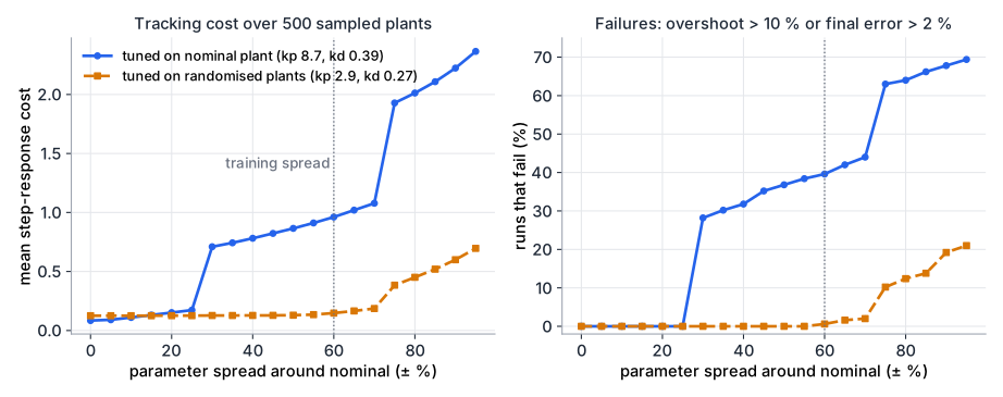
On the nominal plant the nominal gains are better: lower cost, and they reach within 2 % of the target in 0.15 s against 0.39 s. Those gains sit close to the edge. With one extra period of delay, the nominal-tuned loop overshoots by 9.8 % and its cost rises from 0.084 to 1.08. The randomised gains are softer and give up some nominal performance for a much wider safe range. The two approaches meet in practice: identify the robot, then randomise around the identified values over a range set by the measured uncertainty plus what you know you did not model.
For learned policies the recipe is the same, with the policy in place of the gains: randomise physics and rendering for every training episode, and validate on held-out parameter draws before going near hardware.
Simulators in use
MuJoCo (Multi-Joint dynamics with Contact) is a general-purpose physics engine for robotics research. Google DeepMind maintains it as open source under the Apache 2.0 licence. MuJoCo XLA (MJX) runs it under JAX, and MuJoCo Playground builds GPU-accelerated RL training on it. Its original description is the IROS 2012 paper by Todorov, Erez and Tassa, which presents it as an engine tailored to model-based control.
Isaac Sim and Isaac Lab come from NVIDIA. Isaac Lab describes itself as a unified, modular framework for robot learning, with GPU-accelerated physics through PhysX and Newton, photo-realistic scenes and RTX rendering through Isaac Sim, and domain randomisation among its features. It supports workflows for reinforcement learning, learning from demonstrations and motion planning. The framework is open source under the BSD-3-Clause licence, with some parts under Apache 2.0.
For the SO-101, the SO-ARM100 repository publishes a URDF model of the arm, which the LeRobot documentation uses for kinematics. A URDF describes links, joints and limits. Masses, damping and servo behaviour still need identification before simulated dynamics match the real arm.
Vision-language-action models
A VLA is a policy built on a pretrained vision-language model (VLM). The idea is to inherit what the VLM learned from web-scale images and text (objects, spatial words, instructions) and train it further to output robot actions.
- In: one or more camera images, a natural-language instruction such as “put the red cube in the bin”, and usually the robot state (joint positions).
- Out: an action, or an action chunk of several future actions, in the robot’s command space (joint goal positions or end-effector deltas).
The four models below show the main design choices. Each description stays at the level of detail its paper gives.
| Model | Backbone and size | Inputs | Action output |
|---|---|---|---|
| RT-2 (2023) | VLMs co-fine-tuned on robot trajectories and web vision-language tasks | Images, instruction | Actions written as text tokens, trained like language |
| OpenVLA (2024) | 7B parameters: Llama 2 with a visual encoder that fuses DINOv2 and SigLIP features | One image, instruction (no proprioception) | 7 dimensions, each one of 256 bins, as tokens |
| π0 (2024) | 3B PaliGemma VLM plus a 300M action expert (3.3B total) | Several RGB images, language command, proprioceptive state | Continuous actions by flow matching, chunks of H = 50 |
| SmolVLA (2025) | 450M parameters, about 100M in the action expert; SmolVLM-2 backbone | Several RGB images, instruction, sensorimotor state | Continuous actions by flow matching, chunks of n = 50 |
The RT-2 paper named this category of models VLAs. It fits robot actions into the same format as language by writing them as text tokens. A single model is co-fine-tuned on robot trajectories and on web tasks such as visual question answering. The paper reports better generalisation to new objects and to instructions that were not in the robot data.
OpenVLA is open source and was trained on 970k real robot demonstrations. Each action dimension is discretised separately into 256 bins that divide the range between the 1st and 99th percentile of the training actions evenly. The bin indices replace the 256 least used tokens of the Llama tokenizer, and training uses next-token cross-entropy on the action tokens. The paper shows fine-tuning on consumer GPUs with low-rank adaptation (LoRA) and serving with quantisation.
π0 keeps actions continuous. A separate action expert, attached to the VLM, uses conditional flow matching to model the distribution of continuous action chunks of 50 steps. The paper reports control at up to 50 Hz on dexterous tasks such as laundry folding.
SmolVLA is built to be trained on one GPU and run on consumer GPUs or CPUs. It uses only the first 16 layers of the language model inside the VLM, limits each frame to 64 visual tokens, and uses a flow-matching transformer as the action expert. Its pretraining data is fewer than 30k episodes from 481 community datasets on the Hugging Face Hub. It also uses asynchronous inference, which starts predicting the next chunk while the robot still executes the current one. This links back to the action chunking of ACT: chunks hide inference latency and smooth motion.
Size drives deployment. A 7B model needs about 15 times the weight memory and arithmetic per step of a 450M model, which decides whether it can run on the edge hardware discussed in lesson 12.
Fine-tuning SmolVLA on your own data
SmolVLA is a base model. LeRobot’s documentation says fine-tuning on your own data is needed for good performance in your setup. It recommends about 50 episodes as a starting point, with several demonstrations for each variation you introduce. Its reference dataset has 50 episodes over 5 cube positions, 10 per position, and the documentation notes that a similar 25-episode dataset was not enough.
The commands below are taken from the LeRobot SmolVLA documentation as fetched in November 2026, with the dataset and model names replaced by placeholders for your own. They were not run for this lesson. LeRobot changes quickly, so check the current page before you use them.
# Inside a LeRobot source checkout, after the LeRobot installation guide:
pip install -e ".[smolvla]"

lerobot-train \
  --policy.path=lerobot/smolvla_base \
  --dataset.repo_id=${HF_USER}/my_so101_dataset \
  --policy.repo_id=${HF_USER}/my_smolvla \
  --rename_map='{"observation.images.top": "observation.images.camera1", "observation.images.wrist": "observation.images.camera2"}' \
  --batch_size=64 \
  --steps=20000 \
  --output_dir=outputs/train/my_smolvla \
  --job_name=my_smolvla_training \
  --policy.device=cuda \
  --trackio.enable=true
The documentation’s own example trains on lerobot/svla_so100_pickplace; replace it with your dataset. --rename_map maps your camera names to the camera1, camera2 and camera3 names that smolvla_base expects. Without it, training stops with a feature-mismatch error. The documentation gives about 4 hours for 20k steps on a single A100 GPU. Run the trained policy on the follower arm with:
lerobot-rollout \
  --strategy.type=base \
  --robot.type=so101_follower \
  --robot.port=/dev/ttyACM0 \
  --robot.id=my_blue_follower_arm \
  --robot.cameras="{ top: {type: opencv, index_or_path: 0, width: 640, height: 480, fps: 30}, wrist: {type: opencv, index_or_path: 1, width: 640, height: 480, fps: 30}}" \
  --rename_map='{"observation.images.top": "observation.images.camera1", "observation.images.wrist": "observation.images.camera2"}' \
  --task="Grasp a lego block and put it in the bin." \
  --policy.path=${HF_USER}/my_smolvla
Use the same camera names, resolution, --rename_map and task text as in the recording. A different phrasing of the task is a generalisation test, not the training condition. --strategy.type=episodic records evaluation episodes, with an optional teleoperator to reset the scene between them.
Evaluating generalisation
A success rate on the training conditions says little. Plan the evaluation before collecting data, and hold out conditions that never appear in training:
- In-distribution: the training object at the training positions. This is the baseline.
- New positions: the same object at positions between and outside the training positions.
- New objects: different shape, colour or size, with the same instruction.
- New instructions: paraphrases (“drop the block in the box”) and new targets (“the blue block”).
- Disturbances: distractor objects, changed lighting, a moved camera, a nudge during the grasp.
For each condition, run a fixed number of trials with positions set from a list written in advance, and log every trial. Record success or failure, the failure mode (missed grasp, dropped object, wrong object, collision, timeout) and the time to finish. Report counts with an interval, not a bare percentage. For successes in trials, the Wilson 95 % interval is
With 20 trials per condition, the intervals are about ±20 percentage points wide. Only large differences between policies are real at that sample size.
How sure is 14 out of 20?
A fine-tuned policy succeeds in 14 of 20 trials at new positions. Compute the Wilson 95 % interval. Then compute it for 7 of 10. Does the larger test tell you something the smaller one did not?
Show solution
For , : , , so the denominator is 1.1921. The centre is . The half-width is . The interval is about 48 % to 85 %.
For , the same formula gives about 40 % to 89 %. Both tests have the same point estimate. The 20-trial test narrows the interval by about 12 percentage points but still cannot separate this policy from one with a true success rate of 50 %. To tell apart two policies that differ by 10 points you need well over a hundred trials each.
How wide should you randomise?
In domain_rand.py, tune the randomised gains with a training spread of 0.3 and 0.9 instead of 0.6. Before running it, predict how the gains and the nominal cost change. Then evaluate each tuning at spreads 0, 0.3, 0.6 and 0.9.
Show solution
Wider training ranges give softer gains. The run gives , for a spread of 0.3, and , for 0.9 (against 2.87 and 0.268 for 0.6).
| Training spread | Cost at 0 | Fail at 0.6 | Fail at 0.9 |
|---|---|---|---|
| 0.3 | 0.101 | 3.2 % | 35.8 % |
| 0.6 | 0.126 | 0.6 % | 19.2 % |
| 0.9 | 0.313 | 2.2 % | 24.2 % |
Training at 0.3 does well up to its own range and fails beyond it. Training at 0.9 has about 2.5 times the nominal cost of the 0.6 tuning and still fails more often at a spread of 0.9. Most of its failures (98 of 121) are slow responses that are still more than 2 % from the target when the 1.5 s test ends. Over-wide randomisation is not free: it trades performance everywhere for coverage of plants you may never meet. Base the range on measured uncertainty plus a margin.
Summary
- The reality gap has four parts: dynamics, sensing, latency and visuals. On a bus-servo arm, the servo’s internal loop and the command delay often matter as much as the rigid-body parameters.
- System identification fits a model to measured data. Linear least squares gives start values, and Gauss-Newton refines them. Formula-based uncertainties are a lower bound when the noise is not Gaussian.
- Domain randomisation trains or tunes over a distribution of simulated worlds. In the joint example it kept failures near zero up to ±55 % parameter spread, at the price of slower nominal performance.
- MuJoCo and Isaac Lab are the main open simulators for robot learning. Both support GPU-accelerated simulation, and Isaac Lab includes domain randomisation as a feature.
- A VLA maps images, an instruction and robot state to actions or action chunks. RT-2 and OpenVLA emit action tokens, while π0 and SmolVLA generate continuous chunks with flow matching.
- Fine-tune a small VLA such as SmolVLA on about 50 or more episodes that repeat each variation, and evaluate on held-out positions, objects and instructions with counts and confidence intervals.
Check your understanding
Pick an answer for each question, then check. Answers stay hidden until you submit.
Further reading
- Paper
- Paper
- Paper
- Paper
- Paper
- Paper
- Documentation
- Documentation
- Tool
Found a mistake or something unclear?Report a correction.
Follow this course
Get an email when new lessons and projects are added to this course.