Kinematics and control · Lesson 3 of 12
Forward kinematics for robot arms: DH, URDF and the SO-101
Compute where a robot arm's gripper is from its joint angles: a planar 2-link arm by hand, DH tables, product of exponentials, and the SO-101's URDF in NumPy.
What you will learn
- Define joints, links, degrees of freedom, configuration space and workspace for a serial arm
- Compute the tip position of a planar 2-link arm by hand and as a product of transforms
- Write standard and modified Denavit-Hartenberg tables and explain how they differ
- Read joint origins and axes from a URDF and compute forward kinematics for the SO-101
- Compare a learned forward kinematics model with the analytic one and explain when each fits
Before you start
- Spatial maths: rotations and transforms (lesson 2)
After this lesson you can compute where a robot arm’s gripper is from its joint angles. You will do it by hand for a planar 2-link arm, write the same arm as a Denavit-Hartenberg table, and then compute the pose of the SO-101’s gripper from the joint origins and axes in its official URDF file. The last section compares that analytic model with a model fitted to data.
Joints, links and configuration space
A serial arm is a chain of rigid links connected by joints. A revolute joint rotates about an axis; a prismatic joint slides along one. Each of these joints adds one degree of freedom (DOF). The SO-101 has five revolute joints that move the gripper and a sixth that opens it.
Two spaces describe the arm:
- Configuration space (joint space): the vector of joint values . For the SO-101 arm it is five angles, each limited to a range. The URDF limits are ±110° for the shoulder pan, ±100° for the shoulder lift, ±96.8° for the elbow, ±95° for the wrist flex, and −157.2° to +162.8° for the wrist roll.
- Task space: the pose of the gripper, a position and an orientation, written as a transform from the base frame 0 to the end-effector frame E.
Forward kinematics (FK) is the map from configuration space to task space, . It always has exactly one answer. The reverse map, inverse kinematics, may have none, one or many. The workspace is the set of positions the tip can reach.
A planar 2-link arm by hand
Start with two links in a plane. Joint 1 sits at the origin; its angle is measured from the x axis. Joint 2 sits at the end of link 1; its angle is measured relative to link 1. With link lengths and :
where is the elbow and is the tip. The orientation of the last link is .
Worked example. Take m and m, the shoulder-to-elbow and elbow-to-wrist distances in the SO-101 URDF, rounded to the millimetre. Set and .
| Term | Value |
|---|---|
| m | |
| m | |
| m | |
| m | |
| Tip | m |
The tip is 0.232 m from the base, inside the maximum reach of m.
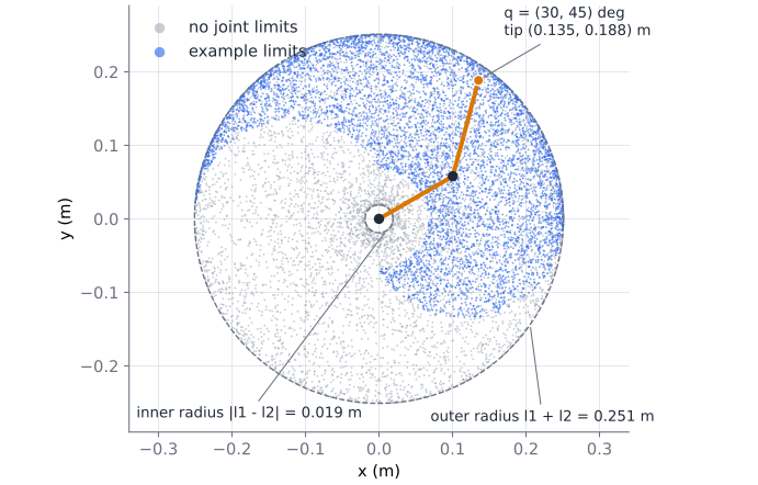
Without limits, the tip can reach any point between m and m from the base. Most points inside the annulus are reached by two configurations, elbow up and elbow down. Joint limits remove one of them in places, and remove whole regions elsewhere. Real workspaces also lose points to collisions with the arm’s own links and the table, which FK alone does not model.
Forward kinematics as a product of transforms
The same arm can be written with the 4×4 transforms from the spatial maths lesson. Rotate about z by , slide along the new x by , rotate by , slide by :
Multiplying out gives the formulas above in the last column, and the rotation block is . This is the pattern for every serial arm: one transform per link, some of them depending on a joint variable, multiplied from base to tip:
The conventions below differ only in how they place the frames and write each factor.
Denavit-Hartenberg parameters
The Denavit-Hartenberg convention, published in 1955 (see further reading), places frames by a few rules so that each link transform needs only four parameters instead of six. Two describe the link: its length and its twist , the distance and angle between consecutive joint axes. Two describe the joint: the offset along the joint axis and the angle about it. A revolute joint varies ; a prismatic joint varies .
Two variants are in common use, and they are not interchangeable:
| Standard (distal) DH | Modified (proximal) DH | |
|---|---|---|
| Frame is attached to | the far end of link , with on the axis of joint | the near end of link , with on the axis of joint |
| Link transform | ||
| Parameters in row | ||
| Last link length | in the table | a separate tool transform |
A DH table from a paper or datasheet is only useful if you know which variant it uses. Mixing them gives a model that is wrong without any error message. For the planar 2-link arm:
| Joint | Standard: | Modified: | ||||||
|---|---|---|---|---|---|---|---|---|
| 1 | 0 | 0 | 0 | 0 | 0 | |||
| 2 | 0 | 0 | 0 | 0 | ||||
| Tool | 0 | 0 | 0 |
The code builds both and the tests check that they give the same tip. DH tables are compact and common in older literature and industrial datasheets. Their weakness is that the frame rules force frames into awkward places for many real arms, and parallel consecutive axes, such as the SO-101 shoulder lift, elbow and wrist flex, make the common normal ambiguous.
Product of exponentials
The product-of-exponentials (POE) formula, the main notation of the textbook Modern Robotics, avoids link frames altogether. Put the arm in its home pose, . For each joint, write its screw axis in the base frame: a unit direction and the vector , where is any point on the axis. Record the home pose of the tool. Then
with given by Rodrigues’ formula. Every joint is treated the same way, the axes can be read straight off a CAD model, and no parameter becomes ambiguous for parallel axes. The test file builds the POE model of the SO-101 from its URDF and checks that it matches the chain of URDF transforms in 50 random configurations.
URDF: the format arms ship with
Most arms, including the SO-101, come with a URDF (Unified Robot Description Format) file. It is XML, with a link element for each rigid body (mass, inertia, meshes for display and collision) and a joint element for each connection. For kinematics only the joints matter. This is the SO-101 elbow joint:
<joint name="elbow_flex" type="revolute">
  <origin xyz="-0.11257 -0.028 1.73763e-16" rpy="-3.63608e-16 8.74301e-16 1.5708"/>
  <parent link="upper_arm_link"/>
  <child link="lower_arm_link"/>
  <axis xyz="0 0 1"/>
  <limit effort="10" velocity="10" lower="-1.69" upper="1.69"/>
</joint>
The URDF specification defines origin as the transform from the parent link frame to the joint frame. Its rpy is roll about x, then pitch about y, then yaw about z, all about fixed axes, which is from the previous lesson. The axis is given in the joint frame. So each joint contributes
Values such as 1.73763e-16 are rounding noise from the CAD export and are effectively zero. Angles such as 1.5708 and 3.14159 are and rounded to five or six digits, which leaves errors of the order of a micrometre in the computed positions. That is far below anything the servos can resolve.
Forward kinematics for the SO-101
The SO-ARM100 repository publishes so101_new_calib.urdf for the follower arm. The values below come from commit 141aea7 of that file. In this “new calibration” model each joint’s zero is the middle of its range, which is the same convention LeRobot’s calibration uses. The chain from base_link to the fixed gripper_frame_link at the tool point is:
| Joint | Origin xyz (m) | Origin rpy (rad) | Axis |
|---|---|---|---|
shoulder_pan | (0.0388, 0, 0.0624) | (π, 0, −π) | z |
shoulder_lift | (−0.0304, −0.0183, −0.0542) | (−π/2, −π/2, 0) | z |
elbow_flex | (−0.1126, −0.0280, 0) | (0, 0, π/2) | z |
wrist_flex | (−0.1349, 0.0052, 0) | (0, 0, −π/2) | z |
wrist_roll | (0, −0.0611, 0.0181) | (π/2, 0.0487, π) | z |
gripper_frame_joint (fixed) | (−0.0079, −0.0002, −0.0981) | (0, π, 0) | none |
The download keeps all the digits from the file. The code is a loop over this table:
def joint_transform(j: Joint, q: float = 0.0) -> Array:
    """Parent-link to child-link transform: T(origin) @ Rot(axis, q)."""
    T = make_T(rpy_to_R(*j.rpy), j.xyz)
    if j.kind == "revolute":
        T = T @ make_T(rot_axis(j.axis, q), np.zeros(3))
    return T


def chain_fk(joints: list[Joint], q: Array) -> list[Array]:
    frames = [np.eye(4)]
    qi = iter(np.asarray(q, dtype=float))
    for j in joints:
        angle = next(qi) if j.kind == "revolute" else 0.0
        frames.append(frames[-1] @ joint_transform(j, angle))
    return frames
Expressed in the base frame at , the joint axes come out simple, even though the URDF origins look arbitrary. The shoulder pan axis points along −z (vertical). The shoulder lift, elbow and wrist flex axes are all parallel to y, so those three joints move the arm in one vertical plane. The wrist roll axis points along −x. The joint origins are at:
| Frame | Position at (m) |
|---|---|
| shoulder lift | (0.069, −0.018, 0.117) |
| elbow | (0.097, −0.018, 0.229) |
| wrist flex | (0.232, −0.018, 0.234) |
| wrist roll | (0.293, 0.000, 0.234) |
| gripper frame | (0.391, 0.000, 0.227) |
At the middle of every range the upper arm points almost straight up and the forearm points forward, horizontally. The shoulder-to-elbow distance is 0.116 m and the elbow-to-wrist distance is 0.135 m, the values used in the 2-link example. With degrees, the code puts the gripper frame at m.
Two checks before you trust this on a real arm. First, the signs: the URDF and LeRobot share the zero point, but you should confirm on your own arm that a positive command moves each joint the way the model predicts. Move one joint at a time by a known amount and watch. Second, the tool point: gripper_frame_link is a reference point near the fingers. If your task needs a different point, such as the tip of a longer printed finger, add your own fixed transform.
Learned versus analytic models
If a network can learn a policy from data, it can also learn FK from measured joint angles and tip positions. The download tries this with a simple model. It samples 500 configurations with both joints between 0 and 90°, adds 1 mm of measurement noise to the tip positions, and fits polynomials in by least squares. It then tests on fresh points inside that range and on points with both joints between 90° and 180°:
| Polynomial degree | Mean error inside range | Mean error outside range |
|---|---|---|
| 2 | 6.27 mm | 566 mm |
| 4 | 0.24 mm | 365 mm |
| 6 | 0.24 mm | 607 mm |
Inside the training range a degree-4 fit is accurate to a fraction of a millimetre, better than the noise in its own training data because it averages over 500 samples. Outside it, the errors exceed the arm’s own reach. A neural network trained on the same data behaves the same way in kind: it interpolates well and extrapolates poorly.
For a rigid arm with a known URDF, the analytic model wins on every count. It is exact everywhere in the joint space, needs no data, has a handful of parameters with physical meaning, and gives exact derivatives for the Jacobian in the next lesson. A learned model makes sense when the geometry is unknown or does not behave like rigid links: soft or cable-driven arms, large gear backlash, links that bend under load, or a camera-measured “tip” whose relation to the joints is hard to model. Even then, the common approach is a hybrid. Keep the analytic chain, fit its few parameters (link lengths, joint offsets) to measured data, and if needed learn only a small residual on top. That keeps the structure that extrapolates and uses data only for what the model misses.
The code
fk.py contains the planar 2-link formula, standard and modified DH, URDF-style joints with a small parser for joint elements, the SO-101 chain, POE with screw axes, and the polynomial fit. test_fk.py has 18 tests: the hand example, special poses and the reach annulus; both DH conventions against the planar formula; a 3-link DH chain; the URDF parser; rigid-body checks on every SO-101 frame; link lengths that do not change with ; a vertical pan axis; wrist roll leaving its own origin fixed; the SO-101 home position; the POE exponential against SciPy’s matrix exponential; POE against the URDF chain; and the learned model inside and outside its range.
fk.py
Download test_fk.py
python fk.py
python -m pytest -q # 18 passedTwo-link poses by hand
For the 2-link arm with m and m, compute the elbow and tip positions for:
- Which of the two tips is closer to the base, and why are their distances the same?
Show solution
- Elbow . The second link points at , so the tip is m.
- Elbow . The second link points at , so the tip is m.
- Both are m from the base. The distance from base to tip depends only on the elbow angle: , and in both cases. The shoulder angle only rotates the result about the base.
Check with planar_2link_fk(np.pi/2, -np.pi/2, 0.116, 0.135).
A DH table for a 3-link planar arm
A planar arm has three revolute joints with parallel z axes and link lengths 0.30 m, 0.20 m and 0.10 m.
- Write its standard DH table.
- Compute the tip position for .
- Write the same arm in modified DH. What extra transform do you need?
Show solution
- Every row has and ; the joint angle is and is the link length: , , .
- The absolute link angles are 20°, 50° and 10°. m and m. In code:
fk_dh([(0, 0.30, 0), (0, 0.20, 0), (0, 0.10, 0)], np.deg2rad([20, 30, -40])). - Modified rows are , , . The last link length, 0.10 m, is not in the table, so you add a tool transform after joint 3.
Summary
- Forward kinematics maps joint values to the tool pose. It always has one answer and is a product of one transform per link, from base to tool.
- A planar 2-link arm reaches , , inside an annulus from to , cut down further by joint limits.
- DH tables describe each link with four parameters. Standard and modified DH order the factors differently and attach frames at different ends of the link, so always check which one a table uses.
- The product of exponentials needs only joint screw axes and a home pose. URDF gives each joint an origin (xyz, fixed-axis rpy) and an axis, so FK is a loop of .
- The SO-101 URDF puts the gripper frame at (0.391, 0, 0.227) m at mid-range, with the shoulder lift, elbow and wrist flex axes parallel.
- A fitted FK model can be accurate inside its training data and badly wrong outside it. For a rigid arm, use the analytic model and fit only its parameters or a small residual.
Check your understanding
Pick an answer for each question, then check. Answers stay hidden until you submit.
Further reading
- Book
- Book
- Paper
- Documentation
- Tool
Found a mistake or something unclear?Report a correction.
Follow this course
Get an email when new lessons and projects are added to this course.