Robot learning · Lesson 8 of 12
Imitation learning: behaviour cloning and DAgger
Train a robot policy from demonstrations: behaviour cloning, compounding errors, DAgger, multimodal data, and recording an SO-101 dataset with LeRobot.
What you will learn
- Frame behaviour cloning as supervised learning on observation-action pairs
- Explain why errors compound in a behaviour-cloned policy and compare the error bounds of behaviour cloning and DAgger
- Implement behaviour cloning and DAgger in NumPy and measure the difference
- Recognise multimodal demonstrations and why mean-squared-error regression fails on them
- Design and record a teleoperated dataset for the SO-101 arm with LeRobot
Before you start
- Forward kinematics (lesson 3)
- Actuators and control (lesson 5)
- Gradient descent and basic neural networks
After this lesson you can train a policy that copies demonstrations, explain why such a policy drifts once it runs on its own, and fix the drift with DAgger. You will run both methods on a small NumPy task, see the difference in numbers, and then plan and record a real dataset with the SO-101 leader and follower arms.
Demonstrations, observations and actions
Imitation learning replaces hand-written control logic with examples. A person performs the task, and the robot records what it saw and what was done at each time step. One recording of the task, from start to end, is an episode. Each episode is a sequence of frames, sampled at a fixed rate.
At each frame you store:
- the observation : what the policy will be allowed to see at run time. On the SO-101 this is the follower’s six joint positions plus one or more camera images.
- the action : what the policy must output. With a leader arm this is the leader’s joint positions, which the follower’s servos then track as targets. Actuators and control covers the position loop inside each servo.
The policy is a function you train. The demonstrator is the expert, written .
Behaviour cloning is supervised learning
Behaviour cloning (BC) treats each frame as an independent training example and fits the policy by regression:
This is the same training loop as any regression problem: batches of pairs, a loss, gradient descent. It is simple, needs no reward function and no simulator, and works well when the demonstrations cover the states the policy will visit. That last condition is where it breaks.
Distribution shift and compounding errors
Supervised learning assumes that training and test samples come from the same distribution. In BC they do not. Training states come from the expert’s trajectories. Test states come from the policy’s own trajectories, and the policy is not perfect.
Suppose the learned policy makes a small error at step 5. The arm is now a few millimetres from where the expert would have been. The demonstrations never show that state, because the expert never made that error, so the policy’s action there is an extrapolation. It is a little worse than before, the next state is a little further off, and so on. Errors feed into the states that produce the next errors.
Ross, Gordon and Bagnell (AISTATS 2011) make this precise. Let be the task horizon, let the task cost per step be bounded in , and let be the policy’s probability of choosing a different action from the expert, measured on the expert’s state distribution. Citing earlier work by Ross and Bagnell, they state that the total cost of the behaviour-cloned policy satisfies
and that the bound is tight: some problems do incur a cost growing with . For their algorithm, DAgger, they prove a bound linear in :
where is the error of the best policy in hindsight on the states the learned policies actually visited, and bounds how much one deviation from the expert can increase the remaining cost. With of order 1, the difference is large. For an episode of decisions and , the quadratic bound allows an extra cost of 25, the linear one about 0.5.
The intuition: an error made early in a BC rollout lasts for the rest of the episode, and there are steps at which to make the first one. The bounds are worst cases, not predictions. The ACT paper reports the matching symptom on real tasks: the behaviour of the earlier methods it compared against degrades significantly towards the end of an episode.
The DAgger algorithm
DAgger (Dataset Aggregation) trains the policy on the states it actually visits. Following Algorithm 3.1 of the paper:
- Start with an empty dataset and any initial policy .
- For iteration :
- Run the mixed policy for steps, several times.
- For every visited state , record the expert’s action .
- Aggregate: .
- Train on all of .
- Return the best on validation.
With the first iteration is plain behaviour cloning from expert demonstrations. The mixing weight is optional; setting it to 0 after the first round is a common choice and is what the code below does.
The catch is step 2.2. The expert must say what it would have done in states it put the robot in, possibly while the robot was doing something else. That is easy when the expert is a program, such as a planner in simulation. It is hard for a person holding a leader arm, which is why practical variants let the human take over only when the robot is about to fail (see below).
Worked example: reaching around an obstacle
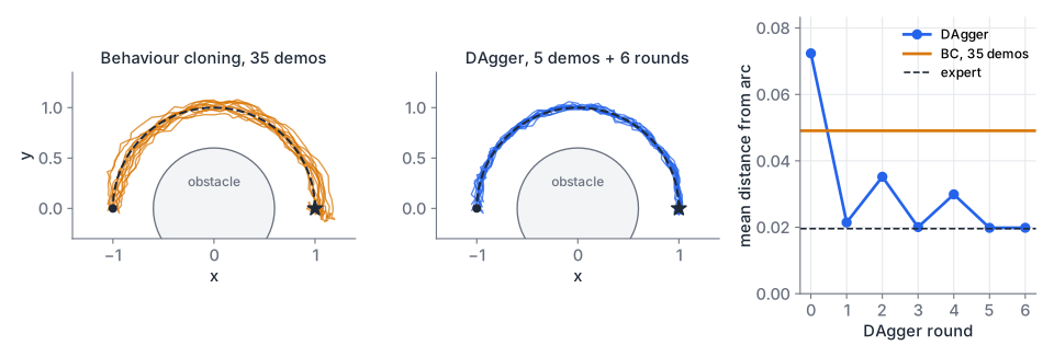
The download reach.py builds a small 2D task where you can see both effects.
- A point robot starts near and must reach . Each step it moves by its action, limited to 0.1, plus Gaussian execution noise.
- The expert follows the upper half of the unit circle, around an obstacle at the origin, at 0.06 per step. Off the arc it also pulls the point back towards radius 1.
- The policy is a small MLP, 2 inputs, 32 tanh units, 2 outputs, trained with full-batch Adam on mean squared error. It sees only the position.
- The expert demonstrations are recorded without execution noise, so they contain almost no recovery behaviour. At deployment the noise standard deviation is 0.02 per step. This exaggerates a real effect: careful human demonstrations rarely show how to recover from a mistake.
The DAgger loop is short:
def dagger(n_demos, n_iters, rollouts_per_iter, seed=0, epochs=2000):
    rng = np.random.default_rng(seed)
    X = collect(expert, n_demos, rng, DEMO_NOISE)
    net = MLP(seed=seed)
    net.fit(X, expert(X), epochs=epochs)
    history = [evaluate(net)["arc_error"]]
    for _ in range(n_iters):
        X_new = collect(net, rollouts_per_iter, rng, EXEC_NOISE)  # states the learner visits
        X = np.vstack([X, X_new])  # aggregate; every state is labelled by the expert below
        net.fit(X, expert(X), epochs=epochs)  # warm start from the previous weights
        history.append(evaluate(net)["arc_error"])
    return net, history
For a fair comparison, BC gets the same number of expert-labelled episodes as DAgger in total: 35. DAgger starts from 5 demonstrations and adds 6 rounds of 5 learner rollouts. Every policy is then evaluated on the same 50 noisy episodes. Arc error is the mean distance from the expert’s arc; success means finishing within 0.1 of the goal.
policy                             arc error  final dist  success
expert                                 0.020       0.023     1.00
BC, 5 demos                            0.072       0.107     0.48
BC, 35 demos                           0.049       0.065     0.82
DAgger, 5 demos + 6 x 5 rollouts       0.020       0.025     1.00
DAgger arc error per round: 0.072 0.021 0.035 0.020 0.030 0.020 0.020
BC action error: 0.0040 on demo states, 0.0267 on its own states
DAgger action error: 0.0029 on demo states, 0.0034 on its own states
Two lines carry the lesson. First, seven times as many demonstrations of the same clean kind only bring BC from 0.072 to 0.049; DAgger reaches the expert’s 0.020. Second, the BC policy’s action error is 0.004 on the states it was trained on and 0.027 on the states it visits itself. That factor of almost 7 is distribution shift, measured. DAgger’s error is about the same on both, because its training set contains its own states.
The per-round history is not monotonic: rounds 2 and 4 are worse than round 1. This is why the algorithm returns the best policy on validation, not simply the last one. This run (seed 0) is the mildest case for BC. Over seeds 0 to 4, BC with 35 demonstrations gave arc errors between 0.049 and 0.365, and DAgger between 0.020 and 0.022.
reach.py
Download test_reach.py
cd public/code/robotics-ai/imitation-learning
/Volumes/M2-Dev/conda/envs/toptech/bin/python reach.py                 # prints the table above
/Volumes/M2-Dev/conda/envs/toptech/bin/python -m pytest -q test_reach.py  # 8 passed
The tests check, on a fixed seed, that DAgger’s arc error is below 0.6 times that of BC, that its final round beats its first, and that BC’s action error on its own states is more than three times its error on demonstration states.
DAgger on a real arm
LeRobot implements a human-in-the-loop variant through lerobot-rollout --strategy.type=dagger. The trained policy drives the follower. When the operator sees an imminent failure, they pause; the leader arm moves to match the follower so there is no jump, and the operator takes control, recovers and corrects. Only the human-controlled segments are recorded by default, and you then fine-tune on the demonstrations plus the corrections. The documentation lists the SO-101 leader as a compatible teleoperator, because the leader’s motors must be able to move to the follower’s pose.
This differs from textbook DAgger. The human labels only the states where they intervene, not every state the policy visits. It is the practical compromise: a person cannot say what they would have done at every frame of a policy run, but they can show a recovery.
The command below is from the LeRobot documentation (v0.7.0), with the SO-101 robot and teleoperator types that the page says to substitute. It was not run here. Ports, IDs and camera indices are placeholders for your setup.
# From the LeRobot documentation, not run here.
lerobot-rollout --strategy.type=dagger \
    --robot.type=so101_follower \
    --robot.port=/dev/tty.usbmodem5AB90687491 \
    --robot.id=my_follower_arm \
    --robot.cameras="{ wrist: {type: opencv, index_or_path: 0, width: 640, height: 480, fps: 30}, top: {type: opencv, index_or_path: 1, width: 640, height: 480, fps: 30}}" \
    --teleop.type=so101_leader \
    --teleop.port=/dev/tty.usbmodem5AB90689011 \
    --teleop.id=my_leader_arm \
    --policy.path=outputs/train/act_so101_test/checkpoints/last/pretrained_model \
    --dataset.repo_id=${HF_USER}/rollout_hil_dataset \
    --dataset.single_task="Grab the black cube" \
    --dataset.fps=30 \
    --strategy.num_episodes=50
During the session, Space pauses and resumes the policy, Tab starts and ends a correction, and Esc stops. Dataset names for lerobot-rollout must start with rollout_.
Multimodal demonstrations
People solve the same task in different ways. One demonstration passes the obstacle on the left, the next on the right; one grasps the mug by the handle, the next by the rim. The action distribution for a given observation then has several modes.
Mean-squared-error regression cannot represent that. For a fixed observation, the action that minimises the expected squared error is the conditional mean . If half the demonstrations have lateral offset and half , the mean is 0: straight into the obstacle, a path no one demonstrated. An L1 loss gives the median instead, which is no better when the two modes have equal weight.
Two remedies:
- Make the data unimodal. Agree on one strategy before recording (always pass on the left, always grasp the handle) and drop episodes that deviate. This is the cheapest fix and usually the first one to try.
- Use a policy that represents several modes. Mixture outputs, generative models such as the conditional VAE in ACT, and diffusion policies can. Action chunking and diffusion policies works through a toy example with numbers.
Designing the dataset
A dataset has a few parameters you choose before you record:
| Parameter | What to decide |
|---|---|
| Frame rate | The control rate of the policy. At 30 fps a 20 s episode is 600 frames. |
| Episode length | Long enough for the slowest successful demonstration, plus a margin. |
| Cameras | Usually one fixed camera with an overview and one on the wrist for the final approach. Fix their mounts. |
| Observation | Joint positions plus images. Record exactly what will be available at deployment. |
| Task description | One string per task, stored with each episode. |
| Initial conditions | A set of object positions and orientations, each covered several times. |
Frames within an episode are strongly correlated, so 50 episodes of 600 frames are far less information than 30 000 independent samples. Diversity comes from episodes.
Teleoperation with a leader arm
The SO-101 leader has the same joint layout as the follower. You move it by hand, and the follower’s servos track its joint positions. The follower uses six STS3215 motors with 1/345 gearing. The leader uses three different gear ratios (1/191, 1/345 and 1/147 on different joints), so it can hold its own weight yet still be moved without much force. Because the joints correspond one to one, the operator gets an intuitive mapping and the recorded action is directly a joint-position target.
Practise before recording. Smooth, consistent motion at a steady speed gives a cleaner dataset than many hesitant episodes.
Recording with LeRobot
The commands below are from the LeRobot documentation (v0.7.0 pages “SO-101” and “Imitation Learning on Real-World Robots”). They were not run here. First check teleoperation alone:
# From the LeRobot documentation, not run here.
lerobot-teleoperate \
    --robot.type=so101_follower \
    --robot.port=/dev/tty.usbmodem58760431541 \
    --robot.id=my_awesome_follower_arm \
    --teleop.type=so101_leader \
    --teleop.port=/dev/tty.usbmodem58760431551 \
    --teleop.id=my_awesome_leader_arm
Then record. The id values select the calibration files, so keep them the same in every step.
# From the LeRobot documentation, not run here.
lerobot-record \
    --robot.type=so101_follower \
    --robot.port=/dev/tty.usbmodem585A0076841 \
    --robot.id=my_awesome_follower_arm \
    --robot.cameras="{ wrist: {type: opencv, index_or_path: 0, width: 640, height: 480, fps: 30}, top: {type: opencv, index_or_path: 1, width: 640, height: 480, fps: 30}}" \
    --teleop.type=so101_leader \
    --teleop.port=/dev/tty.usbmodem58760431551 \
    --teleop.id=my_awesome_leader_arm \
    --display_data=true \
    --dataset.repo_id=${HF_USER}/record-test \
    --dataset.num_episodes=5 \
    --dataset.single_task="Grab the black cube"
Points from the documentation worth knowing:
- The camera names become dataset keys (
observation.images.wrist,observation.images.top). A trained policy expects the same names and resolution at deployment. lerobot-recordappends the date and time to the repository name, for examplerecord-test_20260929_143012, unless you pass--dataset.no_stamp=true.--dataset.episode_time_sand--dataset.reset_time_sset the recording and reset phases (both default to 60 s).- During recording, the right arrow ends an episode early, the left arrow discards and re-records it, and Esc stops the session.
- The dataset is stored as LeRobotDataset v3.0: states and actions in Parquet files, camera frames in MP4 files, and metadata (features, fps, normalisation statistics, episode boundaries) in
meta/. - At the end of a session the tool prints a cadence report. A frame’s timestamp is derived from its index, so a loop that only achieved 25 Hz still produces a dataset that claims 30 fps. Read the report before training.
Replay an episode with lerobot-replay to check that the recorded actions reproduce the motion on the follower.
How many demonstrations
There is no universal number, but there are useful anchors. The LeRobot tutorial suggests at least 50 episodes for a first grasp-and-place task, with 10 episodes per object location, fixed cameras and consistent grasping. The ACT paper recorded 50 demonstrations per real-world bimanual task (100 for one task, Thread Velcro), each 8 to 14 s long at 50 Hz.
Judge your own dataset by measurement, not by count:
- Record 50 episodes over a grid of initial conditions.
- Train on 10, 25 and all 50, with everything else fixed.
- Evaluate each policy on the same set of initial conditions, at least 10 trials each, and record successes per condition.
- If success still rises from 25 to 50 episodes, more data will probably help. If it has flattened, look at the failures instead: a whole region of initial conditions failing points to missing coverage there, scattered failures to noisy or multimodal data.
Validation loss is a poor guide. A lower loss on held-out frames does not guarantee a higher success rate, because the loss is measured on the expert’s states and the robot fails on its own. Lesson 9 shows how to put a confidence interval on a success rate.
Bounds and noise injection
- A task runs for policy steps. On held-out demonstration frames the policy picks a different action from the expert 0.5 % of the time. Evaluate the BC bound and the linear term with . What do the two numbers mean?
- In
reach.py, setDEMO_NOISE = 0.02, so the expert demonstrates with the same execution noise as the deployed policy. Retrain BC with 35 demonstrations. What happens to the arc error and to the distribution-shift numbers, and why?
Show solution
- and . With a cost of 1 per step that differs from the expert, the BC bound allows up to 18 extra bad steps out of 60, while the linear bound allows about one-third of a step. Both are worst cases, but the gap shows why a held-out error rate of 0.5 % does not guarantee a reliable policy.
- With seed 0 the arc error falls from 0.049 to 0.023 and the success rate rises to 1.00. The action error is 0.0065 on demonstration states and 0.0080 on the policy’s own states, a ratio of about 1.2 instead of almost 7. The noisy demonstrations contain the expert’s recoveries from small deviations, so the training data now cover the states the policy drifts into. Perturbing the robot on purpose while recording demonstrations is a cheap alternative to DAgger when it is safe to do so.
import reach
reach.DEMO_NOISE = 0.02
bc = reach.behaviour_cloning(35, seed=0)
print(reach.evaluate(bc), reach.distribution_shift(bc))
Summary
- Behaviour cloning fits by regression on demonstration frames. It is simple and needs no reward, but it trains on the expert’s states and runs on its own.
- Small errors take the policy to unseen states, where errors grow. For supervised imitation the worst-case extra cost grows like ; DAgger’s bound grows like .
- DAgger runs the learner, labels the visited states with the expert’s actions, aggregates and retrains. In the NumPy example it reached the expert’s arc error, while BC with the same number of labelled episodes did not.
- Mean-squared-error regression averages multimodal demonstrations. Record one consistent strategy, or use a policy class that represents several modes.
- With LeRobot,
lerobot-teleoperate,lerobot-recordandlerobot-replaycover teleoperation, recording and checking;lerobot-rollout --strategy.type=daggercollects human corrections. Judge the dataset by success rates across initial conditions, not by validation loss.
Check your understanding
Pick an answer for each question, then check. Answers stay hidden until you submit.
Further reading
- Paper
- Paper
- Paper
- Documentation
- Documentation
- Documentation
- Documentation
Found a mistake or something unclear?Report a correction.
Follow this course
Get an email when new lessons and projects are added to this course.