Perception · Lesson 7 of 12
Deep learning for robot perception: CNNs and detection
How CNNs find objects for a robot arm: convolution and pooling, detector outputs, IoU and NMS, precision, recall and mAP, and a 3D target from a 2D box.
What you will learn
- Compute a 2D convolution, a max-pool and the output size of a convolution layer
- Calculate IoU between two boxes and run non-maximum suppression by hand and in NumPy
- Count true positives, false positives and false negatives and turn them into precision, recall and average precision
- Plan the fine-tuning of a pretrained detector on a small lab dataset
- Convert a 2D detection into a 3D position in the robot base frame with the pinhole camera model
Before you start
- Camera geometry (lesson 6)
- Spatial maths (lesson 2)
- Python and NumPy
After this lesson you can explain what each layer of a convolutional network computes, read the output of an object detector, and score a detector with IoU, precision, recall and average precision. You will also turn a detected box into a 3D target for the SO-101 arm using the camera model from camera geometry, and plan a small labelled dataset for your own lab objects.
From hand-crafted features to learned features
A colour threshold finds a red cube on a white table until the light changes or a second red object appears. Classical vision added hand-designed features, such as gradient histograms and keypoint descriptors, with a trained classifier on top; the features stayed fixed. A convolutional neural network (CNN) learns the features as well, from labelled images. You collect and label data instead of tuning thresholds, and the model only knows what the data showed it.
Convolution, the building block
A convolution layer slides a small kernel of size over the image and takes a weighted sum at every position:
Here is the stride and a bias. Strictly this is cross-correlation: a mathematical convolution flips the kernel first. CNN libraries do not flip, which is harmless for a learned kernel, so in SciPy correlate2d matches a CNN layer and convolve2d does not.
With zero padding on each side, the output length along one axis is
A kernel with , keeps the size. With it halves it: a 640-pixel-wide image becomes 320 wide.
Real layers map input channels to output channels with a weight array; each output map sums the correlations of all input channels with its own kernels. A layer from 64 to 128 channels has parameters, whatever the image size. Compare a fully connected layer from a image to only 1000 units: 921.6 million weights. Weight sharing across positions is what makes CNNs trainable on images.
The download implements this with plain loops and checks it against SciPy:
def conv2d(image, kernel, stride=1, padding=0):
    x = np.asarray(image, dtype=float)
    w = np.asarray(kernel, dtype=float)
    if padding > 0:
        x = np.pad(x, padding, mode="constant")
    kh, kw = w.shape
    oh = (x.shape[0] - kh) // stride + 1
    ow = (x.shape[1] - kw) // stride + 1
    out = np.empty((oh, ow))
    for i in range(oh):
        for j in range(ow):
            r, c = i * stride, j * stride
            out[i, j] = np.sum(x[r : r + kh, c : c + kw] * w)
    return out
On a image with a vertical step from 0 to 1, a Sobel kernel gives 4 in the two output columns whose window straddles the step and 0 elsewhere: an edge detector, much like the kernels a trained first layer learns.
Downloadconv.py
Download test_conv.py
cd public/code/robotics-ai/deep-perception
/Volumes/M2-Dev/conda/envs/toptech/bin/python -m pytest -q test_conv.py
# 10 passed
The tests compare conv2d with scipy.signal.correlate2d, including padding and stride, and confirm that convolve2d gives the flipped-kernel answer.
Nonlinearity and pooling
Stacked linear layers are still one linear map, so each convolution is followed by a nonlinearity, usually the ReLU, . A max pool with stride 2 keeps the largest value in each window, halves the width and height, and tolerates shifts of a pixel or two. Many networks use stride-2 convolutions for the same downsampling. max_pool2d in the download implements pooling.
Feature hierarchies
Each output value depends on a patch of the input called its receptive field. One layer sees 3 pixels across; stacked layers with stride 1 see . Strides and pooling multiply the growth, so after a few downsampling stages a single feature covers a large part of the image. Early layers respond to edges and colour blobs, middle layers to textures and parts, and late layers to whole objects.
The network that turns an image into these features is the backbone. The ACT paper, used in lesson 9, reports that its ResNet-18 backbone maps a image to a feature map: 32 times smaller in each direction, with 512 channels instead of 3.
What a detector outputs
A detector says what is in the image and where. For each object it returns:
- a box, here in pixels with pointing down the image (other tools use centre, width and height);
- a class, such as
cubeorcup; - a score between 0 and 1, the model’s confidence.
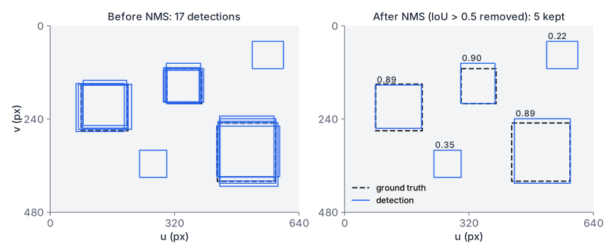
Internally a detector scores many candidate boxes over positions and sizes, from the backbone’s feature maps, either in one pass or by first proposing regions and then classifying them. One object produces several overlapping high-scoring candidates. Post-processing drops boxes below a score threshold, then runs non-maximum suppression.
IoU and non-maximum suppression, with numbers
Intersection over union compares two boxes:
It is 1 for identical boxes and 0 for disjoint ones. Take and . Both are , so each has area 10 000. The intersection runs from to 200 and to 200, which is . The union is , and IoU .
Greedy non-maximum suppression (NMS) works per class:
- Sort the boxes by score.
- Keep the highest-scoring box.
- Remove every remaining box whose IoU with it exceeds a threshold, typically 0.5.
- Repeat with the boxes that are left.
In image processing the same name is used for a pixel-level operation that keeps a pixel only if it is greater than all its neighbours. Neubeck and Van Gool (2006) give fast algorithms for that version, not for box NMS.
Add two boxes to the example: on a second cube, and , another hit on the first cube. The scores are A 0.92, B 0.85, C 0.60, D 0.40. The pairwise IoUs are , , , and 0 for every pair with C. NMS keeps A, removes B and D because both overlap A by more than 0.5, then keeps C. Two boxes remain for two cubes.
def nms(boxes, scores, iou_threshold=0.5):
    b = np.asarray(boxes, dtype=float).reshape(-1, 4)
    order = np.argsort(-np.asarray(scores, dtype=float), kind="stable")
    keep = []
    while order.size > 0:
        best = int(order[0])
        keep.append(best)
        rest = order[1:]
        overlaps = iou_matrix(b[best], b[rest])[0]
        order = rest[overlaps <= iou_threshold]
    return np.array(keep, dtype=np.int64)
The threshold is a trade-off. Too low, and two real objects that touch (two cubes side by side) suppress each other. Too high, and duplicates survive.
Precision, recall and average precision
To score a detector, go through its detections from highest to lowest score. A detection is a true positive (TP) if its IoU with a not-yet-matched ground-truth box of the same class reaches a threshold, often 0.5. Otherwise it is a false positive (FP); a second box on an already matched object is one too. Unmatched ground-truth objects are false negatives (FN).
Precision answers “when the robot reaches for a detection, how often is something there?” Recall answers “of the objects on the table, how many did it find?”
Continue the example with three labelled objects: the two cubes and a third object at that the detector missed. Keep detections with a score of at least 0.5 and skip NMS:
| Setting | TP | FP | FN | Precision | Recall |
|---|---|---|---|---|---|
| Score at least 0.5, no NMS | 2 | 1 | 1 | 0.667 | 0.667 |
| Score at least 0.5, after NMS | 2 | 0 | 1 | 1.000 | 0.667 |
| Score at least 0.9, no NMS | 1 | 0 | 2 | 1.000 | 0.333 |
Box B is the false positive in the first row: a duplicate on cube A. NMS removes it and precision goes to 1. The missed object caps recall at 2/3 regardless of thresholds.
Sweeping the score threshold from high to low traces a precision-recall curve. Average precision (AP) is the area under it, after replacing each precision value by the best precision at the same or any higher recall (the envelope). Mean average precision (mAP) is the mean of AP over classes. Benchmarks differ in the IoU threshold they use, and some average AP over several thresholds, so check the definition before comparing numbers between papers or tools.
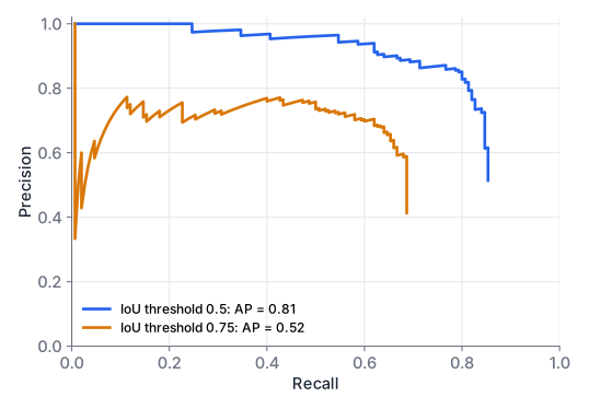
For a robot, pick the operating point from the cost of each error. A false positive sends the gripper to an empty spot; a false negative leaves an object behind. A system that can retry usually favours recall.
Downloadiou.py
Download test_iou.py
iou.py contains iou, iou_matrix, nms, match_detections, precision_recall, pr_curve and average_precision. Running it prints the numbers above, and test_iou.py checks them.
Pretrained backbones and fine-tuning
You rarely train a detector from scratch for a lab task. Backbones pretrained on large labelled image collections already compute general features (edges, textures, object parts). You keep those and train the task-specific layers on your own images. This is fine-tuning. It needs far fewer labelled images than training from scratch, because the network only has to adapt features it already has.
A typical plan:
- Start from a detector pretrained on a large public dataset, with its class head replaced by your classes.
- Freeze the backbone and train only the head. This is fast and hard to overfit.
- Unfreeze the backbone and train everything for a few more epochs with a smaller learning rate (for example ten times smaller), so the pretrained features change slowly.
- Watch validation AP after each epoch and keep the best checkpoint.
Start small, for example 100 labelled images, measure, then add data where the errors are. Split training and validation by recording session, not by random frame. Consecutive video frames are near copies, and a random split puts copies on both sides, which inflates validation scores. Use augmentation: brightness and colour jitter, small scale changes and crops. Flip images only if the task does not depend on left and right.
Segmentation and keypoints
A box around a mug includes table pixels and says nothing about the handle. Two finer outputs are common in manipulation:
- Segmentation labels every pixel. Instance segmentation also separates objects, so two touching cubes get two masks. A mask gives a better centroid and, with depth, a point cloud of just the object. See fully convolutional networks and Mask R-CNN in the further reading.
- Keypoints are named points, such as a mug’s handle. A keypoint network predicts one heatmap per point. Keypoints give orientation, which a box does not, and map directly to grasp points.
Both cost more labelling time per image than boxes.
From a 2D detection to a 3D position
The arm needs a target in metres in its base frame, not a box in pixels. The pinhole model from camera geometry links the two. With intrinsics , a point at depth along the optical axis that projects to pixel lies at
in the camera frame. One pixel gives a ray; the depth has to come from somewhere else. Three common sources:
- A depth camera gives at the pixel directly. Take the median depth over the box or mask, not one pixel, to reject holes and edge noise.
- Known object size. An object of width that appears pixels wide is at , if it faces the camera.
- Known support plane. Objects on a table lie on a plane you can calibrate once. Intersect the pixel ray with the plane .
Worked example with example intrinsics for a image: px, , . The detector returns a box on a 4 cm cube. Its centre is and its width 48 px.
From the size: m, then m and m. This is a point on the cube’s top face, which is what the camera sees.
From the plane: the camera looks straight down from 0.54 m above the table. The cube centre is 2 cm above the table, so intersect the ray with the plane m: m. The two methods agree: a cube on a table 0.54 m away has its top face at 0.50 m. The and values differ slightly because the size method finds the top face and the plane method the centre.
Finally map the point to the base frame with the extrinsic transform from spatial maths: . With the camera at m looking down, the cube centre is at m in the base frame, ready for inverse kinematics.
Downloadlift.py
Download test_lift.py
Data collection and labelling in the lab
- Record what the robot will see: the deployment camera, mount, resolution and lighting. A detector trained on phone photos fails on a wrist camera.
- Vary what will vary: object pose, distractors, daylight at different times, occlusion by the gripper.
- Hold back a test set from a separate session and never tune on it.
- Write a labelling guide first: how tight a box is, whether half-hidden objects count. Label 20 images twice and compute the IoU between the two sets to check consistency.
- Label the model’s failures (missed objects, false positives on shadows) and add them to the training set.
- Keep the provenance: session, camera and date with each image.
IoU, NMS and scoring by hand
A detector returns four boxes for class cube:
| Box | Score | |
|---|---|---|
| P1 | (50, 60, 150, 140) | 0.9 |
| P2 | (60, 70, 160, 150) | 0.8 |
| P3 | (200, 60, 280, 140) | 0.7 |
| P4 | (55, 55, 145, 145) | 0.6 |
The ground truth is and .
- Compute IoU(P1, P2) and IoU(P1, P4).
- Run NMS with a threshold of 0.5. Which boxes are kept?
- Compute precision and recall at IoU 0.5 before and after NMS (all scores are above 0.5).
Show solution
- P1 and P2 are both . The intersection is 60 to 150 and 70 to 140, so . IoU . P4 is ; the intersection with P1 is , so IoU .
- P1 is kept first. P2 (0.650) and P4 (0.809) exceed 0.5 and are removed. P3 does not overlap P1 and is kept. Result: P1 and P3.
- Before NMS: P1 matches (IoU 0.916), P3 matches (IoU 0.841), and P2 and P4 are duplicates on , so TP = 2, FP = 2, FN = 0. Precision , recall . After NMS: TP = 2, FP = 0, FN = 0, so precision and recall are both 1.0.
Check your answers with iou_matrix, nms and precision_recall from iou.py.
How far away is the bottle?
With the same intrinsics as above (, , ), a 6 cm wide bottle is detected with a box 30 px wide centred at .
- Estimate its depth and its position in the camera frame.
- How much does the depth change if the box is one pixel wider or narrower?
Show solution
- m. m and m.
- At 31 px, m; at 29 px, m. One pixel moves the estimate by about 4 cm, about four times the error for the cube at 48 px. Small, distant objects need a depth camera or the table-plane method.
Summary
- A convolution layer slides shared kernels over the input; CNN libraries compute cross-correlation, and the output size is . ReLU and pooling or strided convolutions follow, and stacked layers build features from edges up to objects.
- A detector outputs boxes, classes and scores. A score threshold and per-class non-maximum suppression turn many overlapping candidates into one box per object.
- IoU measures box overlap. With an IoU threshold, detections become true or false positives, and missed objects false negatives. Precision and recall follow, and AP is the area under the precision-recall envelope.
- Fine-tune a pretrained detector instead of training from scratch, split data by session, and add the model’s own failures to the training set.
- A box plus the pinhole model gives a ray; depth from a depth camera, a known object size or a known table plane fixes the point, and the extrinsic transform puts it in the base frame.
Check your understanding
Pick an answer for each question, then check. Answers stay hidden until you submit.
Further reading
- Paper
- Paper
- Paper
- Paper
- Paper
- Paper
- Paper
- Paper
- Documentation
Found a mistake or something unclear?Report a correction.
Follow this course
Get an email when new lessons and projects are added to this course.