Robot learning · Lesson 9 of 12
Action chunking and diffusion policies: ACT and beyond
Why robot policies predict action chunks, how ACT and diffusion policies work, training them with LeRobot, and reporting success rates with a Wilson interval.
What you will learn
- Explain how predicting chunks of k actions reduces compounding errors and smooths motion
- Describe the ACT architecture: CVAE encoder, transformer encoder-decoder and temporal ensembling
- Implement temporal ensembling with exponential weights and show its effect in NumPy
- Explain why diffusion policies represent multimodal action distributions that MSE regression averages away
- Evaluate a policy over N trials and report the success rate with a Wilson score interval
Before you start
- Imitation learning (lesson 8)
- Deep learning for robot perception (lesson 7)
- Basic probability: Bernoulli trials and the normal distribution
After this lesson you can explain the two policy classes most often trained on low-cost arms today, ACT and diffusion policies, and the ideas behind them: predicting chunks of future actions, and modelling a distribution of actions instead of a single mean. You will implement temporal ensembling and a Wilson confidence interval in NumPy, and set up an evaluation that gives success rates you can defend.
Why predict chunks of actions
A single-step policy maps the current observation to the next action, . Lesson 8 showed that its errors compound over the horizon . On an arm controlled at 30 to 50 Hz, a 10 s task is 300 to 500 decisions, each a chance to drift.
An action-chunking policy predicts the next actions at once, , and executes them before it looks again. The ACT paper (Zhao et al., RSS 2023) describes three effects:
- Shorter effective horizon. With one query every steps, a -step task becomes decisions, a -fold reduction.
- Temporal consistency. The actions come out of one forward pass, so they form a coherent motion instead of independent guesses.
- Pauses inside a chunk. Human demonstrations contain pauses and hesitations that depend on time, not on the observation. A single-step policy struggles to model them; inside a chunk the problem is mitigated.
The paper’s ablation, without temporal ensembling and averaged over four simulated settings, shows success rising from 1 % at to 44 % at , then dipping slightly towards fully open-loop control at = 200 and 400. Chunking is not free: while a chunk plays, the policy ignores new observations, and switching chunks every steps causes jumps.
ACT: Action Chunking with Transformers
ACT was designed for low-cost teleoperated arms with a leader-follower setup, the same idea as the SO-101 pair. The paper’s tasks used four cameras and two arms, 14 joint values in total. Actions are absolute target joint positions; the authors report worse results with joint-position deltas.
A conditional VAE
Human demonstrations of the same situation differ. To model that variation, ACT is trained as a conditional variational autoencoder (CVAE) with a latent “style” variable .
- The CVAE encoder is a transformer that reads a learned
[CLS]token, the current joint positions and the demonstrated chunk . It outputs the mean and variance of a diagonal Gaussian over . Images are left out of the encoder to speed up training. - The CVAE decoder is the policy. It takes the images, the joint positions and , and predicts the -step chunk.
- The loss is reconstruction plus times the KL divergence between the encoder’s Gaussian and . The text of the paper states an L1 reconstruction loss, which the authors found more precise than L2.
- At test time the encoder is discarded and is set to the prior mean, zero.
Transformer encoder and decoder
Each camera image goes through a ResNet-18 backbone, which turns a image into a feature map. Flattened, that is 300 tokens of dimension 512 per camera, 1200 for four cameras. With one token each for the joint positions and , the transformer encoder sees 1202 tokens and mixes information across cameras. The transformer decoder uses fixed position embeddings as queries, attends to the encoder output through cross-attention, and an MLP maps the result to joint-position vectors.
The paper’s hyperparameters include and . The model has about 80 M parameters, trained in about 5 hours on one RTX 2080 Ti, with about 0.01 s inference time on the same GPU.
Temporal ensembling
To keep chunking’s consistency without its jumps, ACT queries the policy at every step. Chunks then overlap: at time there are up to predictions for , made at times . Algorithm 2 of the paper averages them with exponential weights:
where is the -th prediction for time and is the oldest. For the oldest prediction has the largest weight. The paper notes that a smaller means faster incorporation of new observations, and that the ensemble adds inference cost but no training cost. For 5 predictions and the normalised weights are .
The implementation keeps a buffer of predictions per future time step:
class TemporalEnsembler:
    def __init__(self, m: float) -> None:
        self.m = m
        self.buffer: defaultdict[int, list[NDArray[np.float64]]] = defaultdict(list)

    def step(self, t: int, chunk: ArrayLike) -> NDArray[np.float64]:
        c = np.atleast_2d(np.asarray(chunk, dtype=float))
        for j, a in enumerate(c):
            self.buffer[t + j].append(a)  # appended in time order, so index 0 is the oldest
        preds = np.array(self.buffer.pop(t))
        return ensemble_weights(len(preds), self.m) @ preds
To see the effect, chunking.py replaces the network with a stand-in: each chunk is a target joint trajectory plus one random offset per chunk (standard deviation 0.03 rad) and small per-step noise (0.005 rad). This mimics a policy whose predictions are right in shape but slightly wrong in level each time it is queried.
execution                  RMS error  mean step  max step
target                        0.0000     0.0100    0.0157
open-loop chunks, k = 20      0.0258     0.0125    0.0962
ensemble, m = 0.01            0.0070     0.0100    0.0245
ensemble, m = 0.1             0.0079     0.0103    0.0239
Open-loop chunks jump by up to 0.096 rad at chunk boundaries, six times the largest step of the target. The ensemble averages up to 20 independent offsets, which cuts the RMS error by a factor of about 3.7 and removes the jumps.
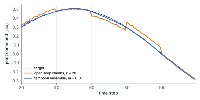
The toy flatters the ensemble in one way. Its offsets are independent between queries and older predictions are as accurate as new ones. On a real robot, a prediction made 99 steps ago used an old observation, so after a disturbance the ensemble reacts slowly; that is the role of . In LeRobot’s ACT configuration, temporal ensembling is controlled by temporal_ensemble_coeff. It defaults to off, requires n_action_steps = 1, and a comment in LeRobot’s code states that the original ACT implementation used 0.01. By default LeRobot’s ACT uses chunk_size = 100 and n_action_steps = 100, so it plays whole chunks.
In the paper’s ablation, temporal ensembling gave ACT a 3.3 % gain in success rate, much less than chunking itself.
Downloadchunking.py
Download test_chunking.py
Multimodal actions: why the mean is wrong
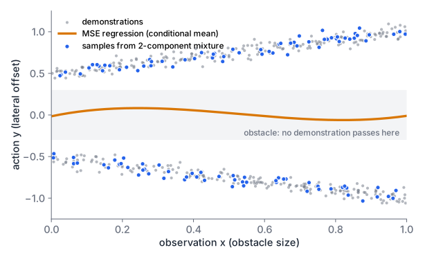
Lesson 8 argued that mean-squared-error regression averages the modes of a multimodal action distribution. bimodal.py shows it with numbers. The observation is an obstacle size between 0 and 1; half the demonstrations pass on the left and half on the right, with lateral offset plus noise of 0.05. No demonstration comes closer than 0.3 to the centre line.
- A cubic polynomial fitted by least squares predicts values between and everywhere. Every prediction lies inside the obstacle band.
- A mixture of two linear-Gaussian components, fitted by expectation maximisation, recovers weights 0.49 and 0.51, slopes and , intercepts and , and spreads of 0.05. Of 1100 samples drawn from it, none falls in the band.
bimodal.py
Download test_bimodal.py
A mixture with a fixed number of Gaussians is one fix. It needs the number of modes in advance and scales poorly to long, high-dimensional action chunks. ACT’s latent is another, although ACT decodes with at test time. Diffusion policies take a third route.
Diffusion policies
A diffusion policy (Chi et al., RSS 2023; extended version in IJRR, 2025) generates an action sequence by starting from noise and removing it step by step, conditioned on the observation.
Denoising as iterative refinement
Write for the action sequence after remaining denoising steps. Sampling starts with drawn from a standard Gaussian and applies, for :
The network predicts the noise in its input. Subtracting it is a small gradient step towards actions that look like the demonstrations; the paper interprets as predicting the gradient of an energy function. , and depend on and form the noise schedule.
Training is simple regression on the noise. Take a demonstrated action sequence and its observation , pick a random step , add noise of the matching size, and minimise
This is mean squared error again, but on the noise, not on the action. The network learns a direction field that points towards the demonstrations from anywhere in action space. Each sample starts from different random noise and slides into one of the modes. The paper attributes the multimodality to exactly these two sources, the random initialisation and the noise added during sampling, and shows a planar pushing task where the diffusion policy commits to going left or right in each rollout, while the baselines either favour one side or switch between them.
The design choices that make it a policy
- Visual conditioning. The observation is an input to , not part of what is generated, so the image encoder runs once per action sequence, not once per denoising step.
- Receding horizon. The policy uses the last observations, predicts future actions, executes the first of them, and then predicts again. This is the same chunking idea as ACT, with replanning built in.
- Network. A 1D temporal CNN conditioned on the observation by FiLM layers, or a transformer. The paper recommends starting with the CNN and switching to the transformer for tasks with fast, sharp action changes.
- Vision encoder. ResNet-18 without pretraining, with spatial softmax pooling instead of global average pooling and GroupNorm instead of BatchNorm, trained end to end.
- Speed. Many denoising steps are slow. With DDIM, the paper trains with 100 steps and runs inference with 10, for 0.1 s latency on an RTX 3080 in its real-world experiments.
The paper also reports that position-control actions worked better than velocity actions with this policy class.
ACT or diffusion
Both predict chunks and both handle multimodal data better than plain regression. ACT needs one forward pass per query and is the policy the LeRobot documentation recommends starting with, citing fast training and good results with about 50 demonstrations. A diffusion policy needs several network evaluations per action sequence, but it represents multimodal action distributions directly. A reasonable plan is to train ACT first, look at the failures, and try a diffusion policy if they come from averaged modes.
Training with LeRobot
The commands below are from the LeRobot documentation and repository (v0.7.0). They were not run here. Training needs a GPU; the documentation shows --policy.device=cuda for NVIDIA cards and mentions mps for Apple silicon.
# From the LeRobot documentation, not run here.
lerobot-train \
  --dataset.repo_id=${HF_USER}/record-test_YYYYMMDD_HHMMSS \
  --policy.type=act \
  --output_dir=outputs/train/act_so101_test \
  --job_name=act_so101_test \
  --policy.device=cuda \
  --policy.repo_id=${HF_USER}/my_policy
Without --steps, training runs for the default 100 000 steps; the documentation notes that imitation learning typically converges within 5 to 10 epochs over the data, so a small dataset needs fewer. Checkpoints go to outputs/train/act_so101_test/checkpoints. The diffusion policy is registered in LeRobot under the type name diffusion, and its extra dependencies are installed with pip install 'lerobot[diffusion]'. Its configuration defaults in v0.7.0 are 2 observation steps, a prediction horizon of 64, 32 executed action steps and 100 DDPM training steps. Switch policies with --policy.type=diffusion and keep the rest of the command.
To evaluate on the arm and record every evaluation episode, the documentation’s episodic rollout strategy runs the policy for a fixed number of episodes with reset phases in between:
# From the LeRobot documentation (SO-100 example; use so101_follower and so101_leader), not run here.
lerobot-rollout \
    --strategy.type=episodic \
    --policy.path=${HF_USER}/my_policy \
    --robot.type=so100_follower \
    --robot.port=/dev/ttyACM0 \
    --teleop.type=so100_leader \
    --teleop.port=/dev/ttyACM1 \
    --dataset.repo_id=${HF_USER}/rollout_eval_data \
    --dataset.num_episodes=20 \
    --dataset.episode_time_s=30 \
    --dataset.reset_time_s=10 \
    --dataset.single_task="Pick up the red cube"
Use the same --robot.id, camera names and task string as in the training data. In simulation, lerobot-eval with --policy.path, --env.type and --eval.n_episodes does the same job.
Evaluating a policy
A success rate from a handful of trials is a noisy number. Treat evaluation as a measurement with a protocol.
The protocol
- Define success before testing, in observable terms: “cube inside the bin and gripper open within 30 s”.
- Fix the initial conditions. Use a grid of object positions, for example 5 positions times 4 trials, and use the same grid for every policy you compare.
- Fix everything else. Same checkpoint, lighting, camera mounts and episode time limit. Randomise the order of trials so that slow drift (warming servos, changing daylight) does not favour one policy.
- Record every trial, including video, and log the outcome before looking at the next one.
- Log failure modes in fixed categories, for example: missed grasp, dropped object, collision, wrong object, timeout, frozen or oscillating. A table of failures by initial condition tells you what to fix: more data at a position, a camera change, or a different policy class.
The ACT paper used 50 trials per seed over 3 seeds in simulation and 25 trials on each real task.
A confidence interval for a success rate
independent trials with successes give the estimate . The textbook (Wald) interval fails at the sample sizes robot experiments use: it can extend past 1, and at 20 out of 20 it collapses to a single point. Use the Wilson score interval instead:
with for 95 %.
Worked example, 18 successes in 20 trials: , , .
- Centre: .
- Half-width: .
- Interval: .
The Wald interval for the same data is . For 20 out of 20, Wilson gives : a perfect run of 20 is still consistent with a true rate as low as 84 %. ACT’s reported 88 % on one real task, from 25 trials (22 successes), has a Wilson interval of .
def wilson_interval(successes: int, n: int, confidence: float = 0.95) -> tuple[float, float]:
    _check(successes, n)
    z = z_value(confidence)
    p = successes / n
    denom = 1.0 + z**2 / n
    centre = (p + z**2 / (2 * n)) / denom
    half = (z / denom) * math.sqrt(p * (1 - p) / n + z**2 / (4 * n**2))
    return max(0.0, centre - half), min(1.0, centre + half)
The test file checks the function against scipy.stats.binomtest(...).proportion_ci(method="wilson") and confirms by simulation that it covers the true rate close to 95 % of the time for , .
stats.py
Download test_stats.py
cd public/code/robotics-ai/act-and-diffusion
/Volumes/M2-Dev/conda/envs/toptech/bin/python -m pytest -q   # 18 passed
To plan the number of trials, use the approximate half-width . For a rate near 80 % and a half-width of 0.1 you need about trials; for 0.05, about 246. Comparisons between two policies need even more, which is why “18/20 versus 15/20” settles nothing (Wilson intervals and ).
Weights and intervals
- At some time step three predictions exist for one joint, oldest first: 0.30, 0.34 and 0.40 rad. Compute the ensembled action for and for . Which one follows the newest prediction more closely?
- Compute the 95 % Wilson intervals for 7 of 10 and 35 of 50 successes. Both estimates are 0.7. What changed?
Show solution
- For the raw weights are , normalised to . The action is rad. For the raw weights are , normalised to , giving rad. The small is closer to the newest value 0.40: it incorporates new observations faster, as the ACT paper states.
- 7/10 gives and 35/50 gives . Five times as many trials shrank the width from 0.495 to 0.247, roughly by . Check with
wilson_interval(7, 10)andwilson_interval(35, 50).
Summary
- Predicting a chunk of actions reduces the effective horizon -fold and gives temporally consistent motion; the ACT paper’s ablation went from 1 % success at to 44 % at .
- ACT is a CVAE: a transformer encoder of joints and the action chunk produces a style variable for training, and a ResNet-plus-transformer decoder predicts the chunk from images, joints and at test time.
- Temporal ensembling queries every step and averages overlapping predictions with weights , oldest first; smaller reacts faster to new observations.
- MSE regression averages modes. A diffusion policy learns to denoise action sequences conditioned on the observation, and each sample commits to one mode; DDIM keeps inference fast enough for control.
- Evaluate with a fixed protocol, log failure modes, and report successes with a Wilson interval: 18/20 is , not “90 %”.
Check your understanding
Pick an answer for each question, then check. Answers stay hidden until you submit.
Further reading
- Paper
- Paper
- Paper
- Paper
- Paper
- Paper
- Documentation
- Documentation
Found a mistake or something unclear?Report a correction.
Follow this course
Get an email when new lessons and projects are added to this course.